
5
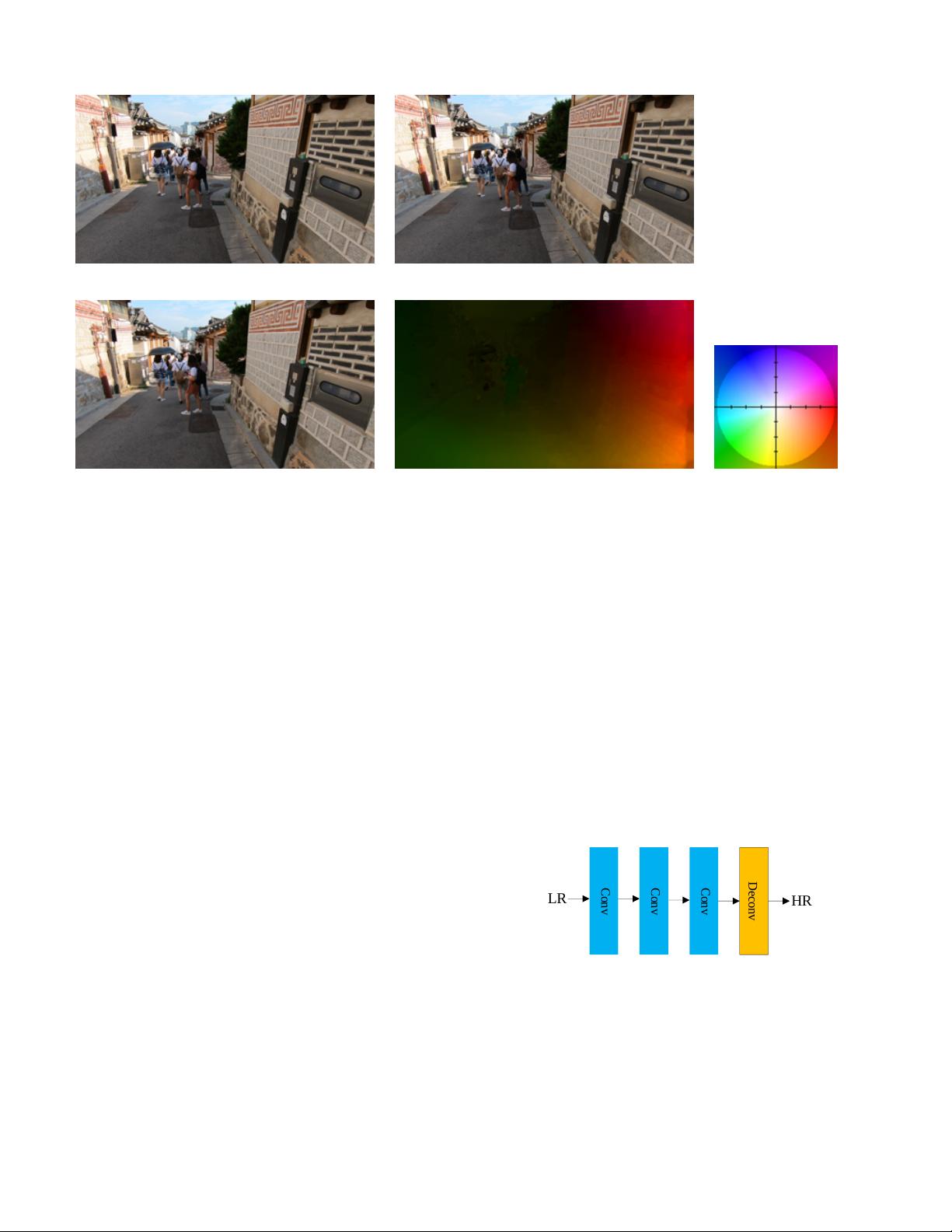
(a) A target frame (b) Its neighboring frame
(c) A compensated image (d) An optical flow image
Fig. 3: An example of motion estimation and compensation. Note that the rightmost image is the legend of (d),
where different colors represent different directions of motion and the intensity of the color denotes the range of
motion.
A. Motion Estimation and Compensation Methods
In the aligned methods for video super-resolution,
most methods apply the motion compensation and mo-
tion estimation techniques. Specifically, the purpose of
motion estimation is to extract inter-frame motion infor-
mation, while motion compensation is used to perform
the warp operation between frames according to inter-
frame motion information and to make one frame align
with another frame. A majority of the motion estimation
techniques are performed by the optical flow method
[45]. This method tries to calculate the motion between
two neighboring frames through their correlations and
variations in the temporal domain. The motion compen-
sation methods can be divided into traditional methods
(such as the LucasKanade [46] and Druleas [47] algo-
rithms) and deep learning methods, such as FlowNet
[45], FlowNet 2.0 [48] and SpyNet [49].
In general, an optical flow method takes two consecu-
tive frames (i.e., I
i
and I
j
) as input, where one is the
target frame and the other is the neighboring frame.
Then the method computes a vector field of optical flow
F
i→j
from the frame I
i
to I
j
by the following formula:
F
i→j
= (h
i→j
, v
i→j
) = M E(I
i
, I
j
; θ
ME
) (10)
where h
i→j
and v
i→j
is the horizontal and vertical com-
ponents of F
i→j
, M E(·) is a function used to compute
optical flow and θ
ME
is its parameter.
The motion compensation is used to perform image
transformation between images in terms of motion infor-
mation to make neighboring frames align with the target
frame spatially. It can be achieved by some methods,
such as bilinear interpolation and spatial transformer
network (STN) [50]. In general, a compensated frame J
is expressed as:
J = M C(I, F ; θ
ME
) (11)
where M C(·) denotes a motion compensation function,
I, F and θ
ME
are the neighboring frame, optical flow
and the parameter, respectively. An example of the mo-
tion estimation and motion compensation is shown in
Fig. 3. Below we depict some representative methods in
this category.
Conv
Conv
Conv
HR
LR
t-n
Alignment module
Non-local
SRNet
HR
VSRResNet
LR
t
LR
t+n
...
......
DNLN
Feature
extraction
LR
t-1
LR
t
Feature
extraction
FRB
HR
LR
FTRN
...
FRB
Dropout
PReLU
RRCN
HRLR
RISTN
Conv
Conv
LR
t-1
LR
t
LR
t+1
......
Conv
...
...
...
LR
t+1
LR
t
LR
t-1
...
...
...
...
Conv
Conv
Conv
Conv
Conv
Conv
...
...
...
...
LR
t
HR
RIB
RIB
RIB
RIB
...
RDC-
LSTM
fusion
Generator
LR
TecoGAN
HR
t-1
HR
t
Upsample
Upsample
...
LR:LR input sequence including LR or upsampled LR
:conv
:motion estimation
:motion compensation :upsample:downsample :3D conv :general resblock
+:element-wise sumc:concat ×: DUF upsample
M. Estim.
Upsample
Upsample
Upsample
M. Comp
Downsample
ResBlock
Conv
Conv
Conv
Conv
Conv
Conv
Conv
Conv
Conv
HR
LR
Conv
Conv
Conv
Deconv
Deep-DE
Fig. 4: The network architecture of Deep-DE [11],
where Conv denotes a convolutional layer and Deconv
denotes a deconvolutional layer.
1) Deep-DE
1
: The deep draft-ensemble learning
method (Deep-DE) [11], as illustrated in Fig. 4, has the
following four major phases. It first generates a series
of SR drafts by adjusting the TV-`
1
loss [51, 52] and
the motion detail preserving (MDP) [53]. Then both
1
Code: http://www.cse.cuhk.edu.hk/leojia/projects/DeepSR/
剩余23页未读,继续阅读

puluowangsi2
- 粉丝: 0
- 资源: 19
 我的内容管理
展开
我的内容管理
展开


最新资源
- 多模态联合稀疏表示在视频目标跟踪中的应用
- Kubernetes资源管控与Gardener开源软件实践解析
- MPI集群监控与负载平衡策略
- 自动化PHP安全漏洞检测:静态代码分析与数据流方法
- 青苔数据CEO程永:技术生态与阿里云开放创新
- 制造业转型: HyperX引领企业上云策略
- 赵维五分享:航空工业电子采购上云实战与运维策略
- 单片机控制的LED点阵显示屏设计及其实现
- 驻云科技李俊涛:AI驱动的云上服务新趋势与挑战
- 6LoWPAN物联网边界路由器:设计与实现
- 猩便利工程师仲小玉:Terraform云资源管理最佳实践与团队协作
- 类差分度改进的互信息特征选择提升文本分类性能
- VERITAS与阿里云合作的混合云转型与数据保护方案
- 云制造中的生产线仿真模型设计与虚拟化研究
- 汪洋在PostgresChina2018分享:高可用 PostgreSQL 工具与架构设计
- 2018 PostgresChina大会:阿里云时空引擎Ganos在PostgreSQL中的创新应用与多模型存储
资源上传下载、课程学习等过程中有任何疑问或建议,欢迎提出宝贵意见哦~我们会及时处理!
点击此处反馈


