
A SURVEY OF LABEL-NOISE REPRESENTATION LEARNING, NOVEMBER 2020 5
TABLE 1
Illustrations of three LNRL examples based on Definition 2.2.
T E = (x, y) P
web-scale image classification (ImageNet, crowdsourced labels) test accuracy
intelligent healthcare (medical data, annotations by variability) error rate
VoIP speech analysis (perceived speech, user feedback) quality rate of voice
which is different with LNRL, where labeled data are still
noisy to some degree. To address SSL, there are several
typical algorithms, such as [27], [48], [48], [49], [50].
•
Positive-unlabeled Learning (PUL) [51] learns the hypothesis
f
from experience
E
consisting of only positive labeled
and unlabeled data. Similar to SSL, unlabeled data will
be normally annotated by pseudo labels. However, PUL
assumes that labeled data are fully clean and only positive.
To address PUL, there are several typical algorithms, such
as [52], [53], [54].
•
Complementary Learning (CL) [55] specifies a class that a
pattern does NOT belong to. Namely, CL learns the hypoth-
esis
f
from experience
E
consisting of only complementary
data. Since the labeling process cannot fully exclude the
uncertainty, namely belonging to which categories, CL
has some relatedness with LNRL. However, CL requires
that all diagonal entries of the transition matrix are zeros.
Sometimes, the transition matrix may be not required to
be invertible in empirical. To address CL, there are several
typical algorithms, such as [55], [56], [57], [58].
•
Unlabeled-unlabeled Learning (UUL) [59] is a recently pro-
posed learning paradigm, which allows us to train a binary
classifier only from two unlabeled datasets with different
class priors. Different to SSL and PUL, there are two sets
of unlabeled data in UUL instead of one set. To address
UUL, there are two typical algorithms, including [59], [60].
3.4 Core Issue
When machine learning in an ideal environment, the data
should be with clean supervision. Therefore,
`
-risk under the
clean distribution should be as follows.
R
`,D
(f
θ
∗
) := E
(X,Y )∼D
[`(f
θ
(X), Y )], (1)
where
(X, Y )
is the clean example i.i.d. drawn from clean
distribution
D
,
f
θ
is a learning model (e.g., a deep neural
network) parameterized by
θ
and
`
is normally cross-entropy
loss. In this survey, we consider the classification problem.
However, when machine learning is in the real-world
environment, the data will be with noisy supervision.
Namely,
`
-risk under the noisy distribution should be
E
(X,
¯
Y )∼
¯
D
[`(f
θ
(X),
¯
Y )]
. Furthermore, under the limited data,
empirical
˜
`
-risk under the noisy distribution should be as
follows.
b
R
˜
`,
¯
D
(f
θ
) :=
1
n
X
n
i=1
˜
`(f
θ
(X
i
),
¯
Y
i
), (2)
where
(X
i
,
¯
Y
i
)
is the (observed) noisy example i.i.d. drawn
from noisy distribution
¯
D
(with noise rate
ρ
). Note that
˜
`
is a suitably modified loss, which is noise-tolerant. Here,
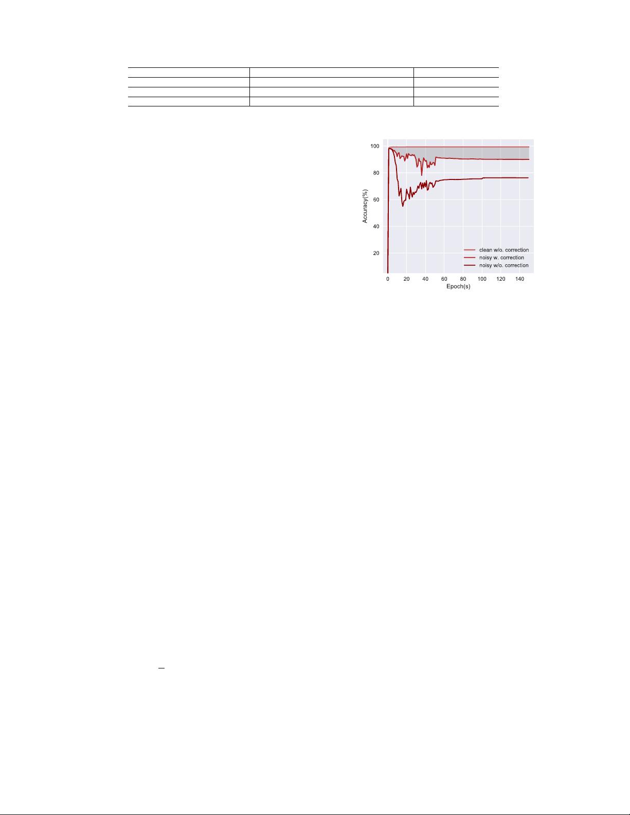
we empirically demonstrate the generalization difference
between ` and
˜
` under label noise (Figure 1).
Generally, the aim of LNRL is to “construct” such noise-
tolerant
˜
`
that the learned
f
θ
in
(2)
approximates to the
Fig. 1. We empirically demonstrate the generalization difference between
original
`
and corrected
˜
`
. We choose MNIST with 35% of uniform noise
as noisy data. There is an obvious gap between
`
and
˜
`
on noisy MNIST.
optimal
f
θ
∗
in
(1)
well. Specifically, via a suitably constructed
˜
`
, we can learn a robust deep classifier
f
θ
from the noisy
training examples that can assign clean labels for test
instances. Before delving into constructing
˜
`
, we first take a
theoretical look at label-noise learning, which will help us
build
˜
` more effectively.
3.5 Theoretical Understanding
In contrast to [9], [10], via the lens of learning theory, we
provide a systematical way to understand LNRL. Our focus
is to explore why noisy labels affect the performance of deep
models. To figure it out, we should rethink the essence of
learning with noisy labels. Normally, there are three key
ingredients in label-noise learning problems, including input
data, objective function and optimization policy.
In high level, there are three rule of thumbs, which explain
how to handle noisy labels effectively via deep models.
•
For data, the key is to discover the underlying noise transi-
tion pattern, which directly links the clean class posterior
and the noisy class posterior. Based on this insight, it
is critical to design unbiased estimator to estimate noise
transition matrix T accurately.
•
For objective function, the key is to design noise-tolerant
˜
`
,
which enjoys the statistical consistency guarantees. Based
on this insight, it is critical to learn a robust classifier on
noisy data, which can provably converge to the learned
classifier on clean data.
•
For optimization policy, the key is to explore the dynamic
process of optimization policies, which relates to mem-
orization. Based on this insight, it is critical to trade-off
overfit/underfit in training deep networks, such as early
stopping and small-loss tricks.
剩余23页未读,继续阅读

syp_net
- 粉丝: 158
- 资源: 1187
 我的内容管理
展开
我的内容管理
展开


最新资源
- AirKiss技术详解:无线传递信息与智能家居连接
- Hibernate主键生成策略详解
- 操作系统实验:位示图法管理磁盘空闲空间
- JSON详解:数据交换的主流格式
- Win7安装Ubuntu双系统详细指南
- FPGA内部结构与工作原理探索
- 信用评分模型解析:WOE、IV与ROC
- 使用LVS+Keepalived构建高可用负载均衡集群
- 微信小程序驱动餐饮与服装业创新转型:便捷管理与低成本优势
- 机器学习入门指南:从基础到进阶
- 解决Win7 IIS配置错误500.22与0x80070032
- SQL-DFS:优化HDFS小文件存储的解决方案
- Hadoop、Hbase、Spark环境部署与主机配置详解
- Kisso:加密会话Cookie实现的单点登录SSO
- OpenCV读取与拼接多幅图像教程
- QT实战:轻松生成与解析JSON数据
资源上传下载、课程学习等过程中有任何疑问或建议,欢迎提出宝贵意见哦~我们会及时处理!
点击此处反馈


