8
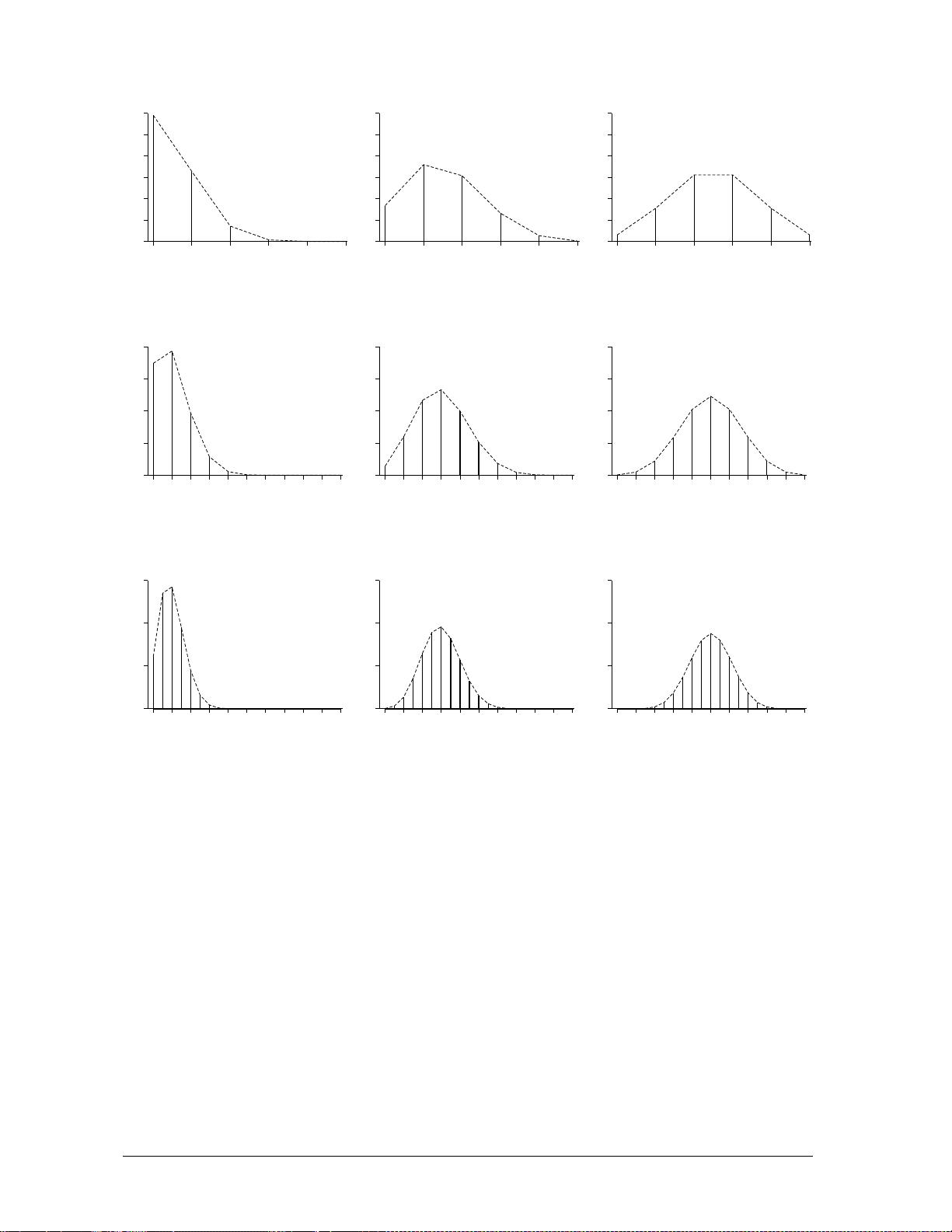
Binomial data are often approximated by a normal distribution.
According to one rule, this is appropriate when both success and failure
mean counts, m
π
and m(1 −
π
), are greater than five. The binomial dis-
tribution is reasonably symmetric and multi-valued when this is the case
(see Figure 2 for m = 20,
π
= 0.3; m = 10,
π
= 0.5; and m = 20,
π
= 0.5).
For various values of
π
, the corresponding minimum sample size required
to use the normal approximation is shown in Table 2.
2
Minimum sample size required to maintain mπ = 5 and corresponding
variance of the binomial distribution
Minimum sample
π
(l −
π
) size, m Variance
0.5 0.5 10 2.5
0.4 0.6 13 3.1
0.3 0.7 17 3.6
0.2 0.8 25 4.0
0.1 0.9 50 4.5
0.05 0.95 100 4.75
0.01 0.99 500 4.95
If
π
is approximately 0.05 or 0.95, then experimental units with approx-
imately 100 sampling units will be required. Therefore, 100 measurements
are needed to determine a mean response for each experimental unit in a
regression or ANOVA. However, the use of familiar statistical methods for
data analysis is a substantial advantage, if such large experiments are feas-
ible. These methods assume homogeneity of variance for all experimental
unit means, which is clearly incorrect for data that are binomially distrib-
uted (since the variance depends on
π
). The angular transformation (i.e.,
arcsine square root) of percentage data is usually recommended to rectify
this situation. For a constant sample size, this transformation will not
make much difference, unless probabilities fall below 0.05 or exceed 0.95,
and data with probabilities of around 0.5 are also present. Occasionally,
the required sample size is so large that the study becomes impractical or
the phenomenon of real interest can not be investigated. Logistic regres-
sion methods use the binomial distribution with its non-constant variance
to model the data. This allows trials to be designed on a smaller scale.
Effects that are only practical or meaningful with smaller sample sizes may
then be studied.
2.3 Logistic Regression
Models
Logistic regression models use the logistic function to fit models to data.
This is an S-shaped function and an example curve is shown in Figure 3.
This function can be used to fit data in three ways. Although each is dis-
tinct, these approaches can be called logistic regression and are briefly
described in Table 3. They all fit a response variable, either y or y/m, to
the S-shaped logistic function of the independent variable, x. The first
model could fit growth data (y on any scale) versus time (x) with a logis-
tic curve, while the next two fit proportional responses (with values
restricted to the range between zero and one) with the logistic curve. The


