混合相机系统线性自校准:中央反射与透视相机的协同解决方案
需积分: 25 140 浏览量
更新于2024-07-09
收藏 920KB PDF 举报
混合中央反射折射和透视相机的自校准是一项针对实际应用中所需多功能相机系统的关键技术。这种混合相机系统结合了大视场和高分辨率的优势,特别适用于需要广角和细节清晰度的场景,如机器人导航、无人机监控和三维成像等。然而,这种混合系统中包含的折反射相机由于其严重的畸变特性,使得精确的校准变得复杂,传统的方法往往依赖于透视相机内参数的先验知识。
本文的主要贡献在于提出了一种创新的自校准方法,解决了混合系统校准问题。该方法突破了既有的限制,不再需要预先知道透视相机的具体内参数,而是通过一种线性校准过程来估计混合相机系统的内参数和外参数。作者采用了一个近似的多项式模型来矫正反射折射图像的畸变,首先利用透视与反射折射图像之间的对极几何关系,线性估计多项式模型的变形参数。然后,通过这个模型,提出了一个新的方法来标定中心反射折射相机,从而实现了相机参数的整体调整。
作者将传统的透视相机的非线性自校准过程简化为线性步骤,提高了整个系统的标定效率。这种方法的优势不仅体现在其灵活性上,还在于其稳健性和可靠性,能够在实际应用中提供准确的相机参数估计,从而提高混合相机系统的整体性能。
实验结果验证了新方法的有效性,展示了其在混合相机系统中的优越性能。这项研究对于推动中央反射折射相机技术的发展,提升三维成像质量和可靠性具有重要意义,为未来的智能设备和视觉系统设计提供了重要的理论支撑。
ular to the line defined by the viewpoints O and O
c
. The angle
u
is
called the view angle of m. The image formation process can be
explicitly expressed as follows [39]:
km ¼ K ðX
s
þð0; 0; nÞ
T
Þð2Þ
K ¼
rf s u
0
0 f
v
0
001
0
B
@
1
C
A
; X
s
¼
RX þ t
kRX þ tk
;
k ¼
n þ
ffiffiffiffiffiffiffiffiffiffiffiffiffiffiffiffiffiffiffiffiffiffiffiffiffiffiffiffiffiffiffiffiffiffiffiffiffiffiffiffiffiffiffiffiffiffiffiffiffiffiffiffiffiffiffi
n
2
m
T
K
T
K
1
mðn
2
1Þ
q
m
T
K
T
K
1
m
ð3Þ
where (R,t), called the extrinsic parameters, is the rotation and
translation which relates the world coordinate system to the view
sphere coordination system O xyz, and K is the camera intrinsic
matrix, with f the focal length, r the aspect ratio, s the skew factor
and p =(u
0
,
v
0
,1)
T
is defined as the homogenous coordination of
the principal point. n is usually called as the mirror parameter,
which is the distance from O to O
c
.Ifn = 1, the used mirror is a
paraboloid (i.e. the camera is paracatadioptric). If 0 < n < 1, the mir-
ror is an ellipsoid or a hyperboloid (i.e. the camera is hypercatadiop-
tric). Since the calibration of a catadioptric camera with n = 0 is the
same with that of a pinhole camera, in this work we only concen-
trate on the calibration of central catadioptric camera with
0<n 6 1.
For the revolution conic section mirror, the mirror parameter n
satisfies [35,1]
n ¼
2
e
1 þ
e
2
ð4Þ
where
e
is the eccentricity of the conic. The relationship between
eccentricity
e
and the mirror parameter n for different types of cen-
tral catadioptric cameras is shown in Table 1 [35]. Generally speak-
ing, the mirror parameter n can be computed easily with the
provided eccentricity
e
from manufactures [1,15,12]. Therefore, n
is assumed to be known in this paper.
For a central catadioptric camera, the principal point can be eas-
ily calibrated using the center of the bounding ellipse [13,35,12] or
line images [32,39,38], and then the origin of the image can be
translated to p by a linear transformation:
T
p
¼
10u
0
01
v
0
00 1
0
B
@
1
C
A
ð5Þ
Hence, the image coordination m can be translated to
~
m by
~
m ¼ T
p
m ¼ðu u
0
;
v
v
0
; 1Þ
T
, and p is translated to
~
p ¼ð0; 0; 1Þ
T
.
Denote
e
K as
e
K ¼
rf s 0
0 f 0
001
0
B
@
1
C
A
ð6Þ
The image formation process (2) can be described by
k
~
m ¼
e
KðX
s
þð0; 0; nÞ
T
Þð7Þ
The matrix
e
K
T
e
K
1
is in the following form:
k
1
k
2
=20
k
2
=2 k
3
0
001
0
B
@
1
C
A
ð8Þ
where
k
1
¼ 1=ðr
2
f
2
Þ; k
2
¼2s=ðr
2
f
3
Þ; k
3
¼ðr
2
f
2
þ s
2
Þ=ðr
2
f
4
Þð9Þ
In this paper, we assume the principal point of catadioptric
camera is precalibrated using the center of the bounding ellipse
like in [39]. Hereafter, denote u , u u
0
;
v
,
v
v
0
; m ,
~
m and
p ,
~
p for simplicity.
2.3. Projective reconstruction by factorization
Suppose there are N perspective cameras P
i
, i =1,..., N and M
3D points X
j
=(X
j
, Y
j
, Z
j
,1)
T
, j =1,..., M. The image coordinates
are represented by m
ij
=(u
ij
,
v
ij
,1)
T
. The image formation process
can be described as follows:
k
ij
m
ij
¼ P
i
X
j
ð10Þ
where k
ij
is a non-zero scale factor, commonly called as the projec-
tive depth.
We stack Eq. (10) of all the cameras into a matrix W
3NM
, which
can be factorized as follows:
k
11
m
11
k
12
m
12
... k
1M
m
1M
k
21
m
21
k
22
m
22
... k
2M
m
2M
... ... ... ...
k
N1
m
N1
k
N2
m
N2
... k
NM
m
NM
0
B
B
B
@
1
C
C
C
A
|fflfflfflfflfflfflfflfflfflfflfflfflfflfflfflfflfflfflfflfflfflfflfflfflfflfflfflfflfflfflfflfflfflfflfflffl{zfflfflfflfflfflfflfflfflfflfflfflfflfflfflfflfflfflfflfflfflfflfflfflfflfflfflfflfflfflfflfflfflfflfflfflffl}
W
3NM
¼
P
1
...
P
N
0
B
@
1
C
A
|fflfflfflffl{zfflfflfflffl}
M
3N4
ðX
1
; ...; X
M
Þ
|fflfflfflfflfflfflfflfflffl{zfflfflfflfflfflfflfflfflffl}
S
4M
ð11Þ
W
3NM
¼ M
3N4
S
4M
ð12Þ
where W is the scaled measurement matrix, M
3N4
¼
P
T
1
; P
T
2
; ...; P
T
N
T
is the projective matrix, and S
4M
=(X
1
, ...,X
M
)is
the projective shape matrix. We use Sturm and Triggs’ method
[28] for the computation of {k
ij
}, and recovery of projective
reconstruction fP
i
g
N
i¼1
by factorizing W. Obviously, the factorization
in (11) is a projective reconstruction up to a 4 4 homography
matrix H
44
. That is, W can also be factorized as W ¼
ðM
3N4
H
44
Þ H
1
44
S
4M
. In order to get the Euclidean reconstruc-
tion, metric constraint should be used to recover the 4 4 homog-
raphy matrix H [16].
3. Calibration method
In this paper, we assume the principal point of catadioptric
camera is precalibrated using the center of the bounding ellipse
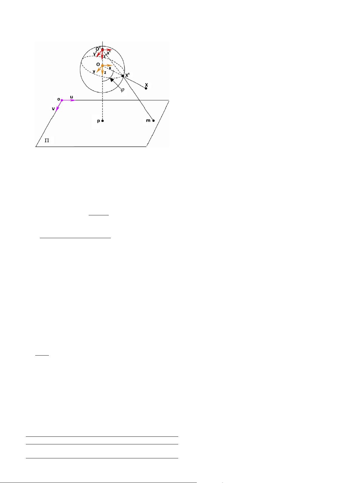
Fig. 1. Image formation of a central catadioptric camera.
Table 1
The relationship between eccentricity
e
and mirror parameter n.
Ellipsoidal Paraboloidal Hyperboloidal Planar
e
0<
e
<1
e
=1
e
>1
e
? 1
n 0<n <1 n =1 0<n <1 n =0
X. Deng et al. / Computer Vision and Image Understanding 116 (2012) 715–729
717
剩余14页未读,继续阅读
2022-07-13 上传
2011-04-28 上传
2024-04-17 上传
2023-06-03 上传
2023-05-10 上传
2023-05-16 上传
2023-05-10 上传
2023-05-15 上传
2023-07-28 上传

weixin_38524246
- 粉丝: 6
- 资源: 920
 我的内容管理
展开
我的内容管理
展开


最新资源
- 计算机人脸表情动画技术发展综述
- 关系数据库的关键字搜索技术综述:模型、架构与未来趋势
- 迭代自适应逆滤波在语音情感识别中的应用
- 概念知识树在旅游领域智能分析中的应用
- 构建is-a层次与OWL本体集成:理论与算法
- 基于语义元的相似度计算方法研究:改进与有效性验证
- 网格梯度多密度聚类算法:去噪与高效聚类
- 网格服务工作流动态调度算法PGSWA研究
- 突发事件连锁反应网络模型与应急预警分析
- BA网络上的病毒营销与网站推广仿真研究
- 离散HSMM故障预测模型:有效提升系统状态预测
- 煤矿安全评价:信息融合与可拓理论的应用
- 多维度Petri网工作流模型MD_WFN:统一建模与应用研究
- 面向过程追踪的知识安全描述方法
- 基于收益的软件过程资源调度优化策略
- 多核环境下基于数据流Java的Web服务器优化实现提升性能
