没有合适的资源?快使用搜索试试~ 我知道了~
首页FPGA技术驱动的神经网络实现进展
《FPGA实现神经网络》是一本由Amos R. Omondi、Jagath C. Rajapakse和Mariusz Bajger编辑的书籍,收录了12篇经过审阅的论文,聚焦于在FPGA(Field-Programmable Gate Array)平台上实现神经网络的研究与实践。该书背景起始于20世纪80年代和90年代初期,当时虽然在硬件神经计算机的设计和实施上投入了大量努力,但这些尝试大多未能取得广泛的成功,主要原因在于当时的ASIC(Application-Specific Integrated Circuit)技术主要针对特定领域,不具备足够的开发成熟度和竞争力,无法支持大规模的应用。 FPGA技术的进步使得当前的FPGA具有足够的容量和性能,成为实现神经网络的理想选择。书中前四章探讨了基础理论和概念,涉及神经网络的原理、FPGA的优势以及设计原则。接着,第五至第十一章深入研究了各种不同的FPGA神经网络实现策略,包括但不限于架构设计、算法优化、硬件加速等,这些章节展示了如何利用FPGA的灵活性和可编程特性来高效地模拟神经网络的计算过程。 最后,第十二章总结了一个大型项目的教训,并结合当前和未来的技术趋势重新审视了设计问题。这一章强调了在实际应用中如何权衡硬件资源、性能和成本,以及如何通过不断的技术进步改进神经网络在FPGA上的部署效率。 《FPGA实现神经网络》是一本实用的参考文献,不仅回顾了过去的努力,也展示了FPGA技术如何推动神经网络硬件的发展,使之成为现代人工智能领域的重要研究方向。通过阅读这本书,读者将能够深入了解FPGA在神经网络中的潜力,并掌握如何利用这种技术进行高效、灵活且成本效益高的计算。
资源详情
资源推荐
4 FPGA Neurocomputers
represented by a set of weights, here denoted by w =(w
1
,w
2
,...w
I
)
T
; and
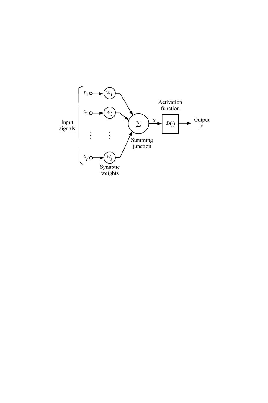
(3) an activation function Φ that relates the total synaptic input to the output
(activation) of the neuron. The main components of an artificial neuron is
illustrated in Figure 1.
Figure 1: The basic components of an artificial neuron
The total synaptic input, u, to the neuron is given by the inner product of the
input and weight vectors:
u =
I
i=1
w
i
x
i
(1.1)
where we assume that the threshold of the activation is incorporated in the
weight vector. The output activation, y,isgivenby
y =Φ(u) (1.2)
where Φ denotes the activation function of the neuron. Consequently, the com-
putation of the inner-products is one of the most important arithmetic opera-
tions to be carried out for a hardware implementation of a neural network. This
means not just the individual multiplications and additions, but also the alterna-
tion of successive multiplications and additions — in other words, a sequence
of multiply-add (also commonly known as multiply-accumulate or MAC) op-
erations. We shall see that current FPGA devices are particularly well-suited
to such computations.
The total synaptic input is transformed to the output via the non-linear acti-
vation function. Commonly employed activation functions for neurons are
Review of neural-network basics 5
the threshold activation function (unit step function or hard limiter):
Φ(u)=
1.0, when u>0,
0.0, otherwise.
the ramp activation function:
2
Φ(u)=max{0.0, min{1.0,u+0.5}}
the sigmodal activation function, where the unipolar sigmoid function is
Φ(u)=
a
1+exp(−bu)
and the bipolar sigmoid is
Φ(u)=a
1 − exp(−bu)
1+exp(−bu)
where a and b represent, repectively, real constants the gain or amplitude
and the slope of the transfer function.
The second most important arithmetic operation required for neural networks
is the computation of such activation functions. We shall see below that the
structure of FPGAs limits the ways in which these operations can be carried
out at reasonable cost, but current FPGAs are also equipped to enable high-
speed implementations of these functions if the right choices are made.
A neuron with a threshold activation function is usually referred to as the
discrete perceptron, and with a continuous activation function, usually a sig-
moidal function, such a neuron is referred to as continuous perceptron. The
sigmoidal is the most pervasive and biologically plausible activation function.
Neural networks attain their operating characteristics through learning or
training. During training, the weights (or strengths) of connections are gradu-
ally adjusted in either supervised or unsupervised manner. In supervised learn-
ing, for each training input pattern, the network is presented with the desired
output (or a teacher), whereas in unsupervised learning, for each training input
pattern, the network adjusts the weights without knowing the correct target.
The network self-organizes to classify similar input patterns into clusters in
unsupervised learning. The learning of a continuous perceptron is by adjust-
ment (using a gradient-descent procedure) of the weight vector, through the
minimization of some error function, usually the square-error between the de-
sired output and the output of the neuron. The resultant learning is known as
2
In general, the slope of the ramp may be other than unity.
6 FPGA Neurocomputers
as delta learning: the new weight-vector, w
new
, after presentation of an input
x and a desired output d is given by
w
new
= w
old
+ αδx
where w
old
refers to the weight vector before the presentation of the input and
the error term, δ,is(d − y)Φ
(u), where y is as defined in Equation 1.2 and
Φ
is the first derivative of Φ. The constant α, where 0 <α≤ 1, denotes the
learning factor. Given a set of training data, Γ={(x
i
,d
i
); i =1,...n}, the
complete procedure of training a continuous perceptron is as follows:
begin: /* training a continuous perceptron */
Initialize weights w
new
Repeat
For each pattern (x
i
,d
i
) do
w
old
= w
new
w
new
= w
old
+ αδx
i
until convergence
end
The weights of the perceptron are initialized to random values, and the conver-
gence of the above algorithm is assumed to have been achieved when no more
significant changes occur in the weight vector.
1.2.2 Multi-layer perceptron
The multi-layer perceptron (MLP) is a feedforward neural network consist-
ing of an input layer of nodes, followed by two or more layers of perceptrons,
the last of which is the output layer. The layers between the input layer and
output layer are referred to as hidden layers. MLPs have been applied success-
fully to many complex real-world problems consisting of non-linear decision
boundaries. Three-layer MLPs have been sufficient for most of these applica-
tions. In what follows, we will briefly describe the architecture and learning of
an L-layer MLP.
Let 0-layer and L-layer represent the input and output layers, respectively;
and let w
l+1
kj
denote the synaptic weight connected to the k-th neuron of the
l +1layer from the j-th neuron of the l-th layer. If the number of perceptrons
in the l-th layer is N
l
, then we shall let W
l
= {w
l
kj
}
N
l
xN
l−1
denote the matrix
of weights connecting to l-th layer. The vector of synaptic inputs to the l-th
layer, u
l
=(u
l
1
,u
l
2
,...u
l
N
l
)
T
is given by
u
l
= W
l
y
l−1
,
where y
l−1
=(y
l−1
1
,y
l−1
2
,...y
l−1
N
l−1
)
T
denotes the vector of outputs at the l−1
layer. The generalized delta learning-rule for the layer l is, for perceptrons,
Review of neural-network basics 7
given by
W
new
l
= W
old
l
+ αδ
l
y
T
l−1
,
where the vector of error terms, δ
T
l
=(δ
l
1
,δ
l
2
,...,δ
l
N
l
) at the l th layer is
given by
δ
l
j
=
2Φ
l
j
(u
l
j
)(d
j
− o
j
), when l = L,
Φ
l
j
(u
l
j
)
N
l+1
k=1
δ
l+1
k
w
l+1
kj
, otherwise,
where o
j
and d
j
denote the network and desired outputs of the j-th output
neuron, respectively; and Φ
l
j
and u
l
j
denote the activation function and total
synaptic input to the j-th neuron at the l-th layer, respectively. During train-
ing, the activities propagate forward for an input pattern; the error terms of a
particular layer are computed by using the error terms in the next layer and,
hence, move in the backward direction. So, the training of MLP is referred as
error back-propagation algorithm. For the rest of this chapter, we shall gen-
eraly focus on MLP networks with backpropagation, this being, arguably, the
most-implemented type of artificial neural networks.
Figure 2: Architecture of a 3-layer MLP network
8 FPGA Neurocomputers
1.2.3 Self-organizing feature maps
Neurons in the cortex of the human brain are organized into layers of neu-
rons. These neurons not only have bottom-up and top-down connections, but
also have lateral connections. A neuron in a layer excites its closest neigh-
bors via lateral connections but inhibits the distant neighbors. Lateral inter-
actions allow neighbors to partially learn the information learned by a winner
(formally defined below), which gives neighbors responding to similar pat-
terns after learning with the winner. This results in topological ordering of
formed clusters. The self-organizing feature map (SOFM) is a two-layer self-
organizing network which is capable of learning input patterns in a topolog-
ically ordered manner at the output layer. The most significant concept in a
learning SOFM is that of learning within a neighbourhood around a winning
neuron. Therefore not only the weights of the winner but also those of the
neighbors of the winner change.
The winning neuron, m, for an input pattern x is chosen according to the
total synaptic input:
m = arg max
j
w
T
j
x,
where w
j
denotes the weight-vector corresponding to the j-th output neuron.
w
T
m
x determines the neuron with the shortest Euclidean distance between its
weight vector and the input vector when the input patterns are normalized to
unity before training.
Let N
m
(t) denote a set of indices corresponding to the neighbourhood size
of the current winner m at the training time or iteration t. The radius of N
m
is
decreased as the training progresses; that is, N
m
(t
1
) > N
m
(t
2
) > N
m
(t
3
) ...,
where t
1
<t
2
<t
3
.... The radius N
m
(t =0)can be very large at the
beginning of learning because it is needed for initial global ordering of weights,
but near the end of training, the neighbourhood may involve no neighbouring
neurons other than the winning one. The weights associated with the winner
and its neighbouring neurons are updated by
∆w
j
= α(j, t)(x − w
j
) for all j ∈N
m
(t),
where the positive learning factor depends on both the training time and the
size of the neighbourhood. For example, a commonly used neighbourhood
function is the Gaussian function
α(N
m
(t),t)=α(t)exp
−
r
j
− r
m
2
2σ
2
(t)
,
where r
m
and r
j
denote the positions of the winning neuron m and of the
winning neighbourhood neurons j, respectively. α(t) is usually reduced at a
剩余364页未读,继续阅读
安全验证
文档复制为VIP权益,开通VIP直接复制
信息提交成功