Matlab Axis Scaling Guide: Flexible Adjustment for Precise Data Presentation
发布时间: 2024-09-13 22:17:14 阅读量: 57 订阅数: 30 

MATLAB 绘图复刻五:带树状图的环形热图
# Matlab Coordinate Axis Scaling Guide: Flexible Adjustment for Precise Data Presentation
 or simultaneously to both axes. Depending on the direction of scaling, there are several types of scaling:
- **x-axis scaling:** Adjusts the range of the x-axis to zoom in or out on the horizontal direction data.
- **y-axis scaling:** Adjusts the range of the y-axis to zoom in or out on the vertical direction data.
- **Dual-axis scaling:** Adjusts the ranges of both the x-axis and y-axis simultaneously to zoom in or out on the data display in two-dimensional space.
### 2.2 Mathematical Representation of Scaling Transformations
Coordinate axis scaling can be represented mathematically through transformation matrices. The scaling transformation matrix `T` is defined as follows:
```
T = [Sx 0 0 0;
0 Sy 0 0;
0 0 1 0;
0 0 0 1]
```
Where:
- `Sx` and `Sy` are the scaling factors for the x-axis and y-axis, respectively.
- `0` elements indicate no shear or rotation transformations.
The scaling transformation matrix `T` is multiplied by the original coordinate points `(x, y)` to obtain the scaled coordinate points `(x', y')`:
```
[x'; y'; 1; 1] = T * [x; y; 1; 1]
```
The values of the scaling factors `Sx` and `Sy` determine the extent of the scaling. When `Sx > 1` and `Sy > 1`, the coordinate axes are enlarged. When `Sx < 1` and `Sy < 1`, the coordinate axes are reduced.
## 3.1 Scaling the Coordinate Axes Using the xlim and ylim Functions
The `xlim` and `ylim` functions are the most basic and commonly used functions for scaling the coordinate axis range. They are used to set the minimum and maximum values for the x-axis and y-axis, respectively.
**Syntax:**
```matlab
xlim([xmin, xmax])
ylim([ymin, ymax])
```
**Parameters:**
- `xmin`: The minimum value of the x-axis
- `xmax`: The maximum value of the x-axis
- `ymin`: The minimum value of the y-axis
- `ymax`: The maximum value of the y-axis
**Code Example:**
```matlab
% Set the x-axis range to [0, 10]
xlim([0, 10]);
% Set the y-axis range to [-5, 5]
ylim([-5, 5]);
```
**Logical Analysis:**
The `xlim` and `ylim` functions scale the coordinate axis range by setting the minimum and maximum values of the axes. When `xmin` and `xmax` are equal, the x-axis is scaled to a single point. Similarly, when `ymin` and `ymax` are equal, the y-axis is scaled to a single point.
### 3.2 Setting the Coordinate Axis Range Using the axis Function
The `axis` function provides a more general method for setting the coordinate axis range. It can set the minimum and maximum values for both the x-axis and y-axis at once, and it can also set the axis ticks and labels.
**Syntax:**
```matlab
axis([xmin, xmax, ymin, ymax])
```
**Parameters:**
- `xmin`: The minimum value of the x-axis
- `xmax`: The maximum value of the x-axis
- `ymin`: The minimum value of the y-axis
- `ymax`: The maximum value of the y-axis
**Code Example:**
```matlab
% Set the coordinate axis range to [0, 10] x [-5, 5]
axis([0, 10, -5, 5]);
```
**Logical Analysis:**
The `axis` function scales the coordinate axis range by setting the minimum and maximum values, ticks, and labels. It offers more flexible control than the `xlim` and `ylim` functions, allowing multiple axis properties to be set in a single command.
### 3.3 Customizing Coordinate Axis Attributes Using the set Function
The `set` function can be used to customize various attributes of the coordinate axis, including range, ticks, labels, grid lines, and titles.
**Syntax:**
```matlab
set(gca, 'PropertyName', PropertyValue)
```
**Parameters:**
- `gca`: The current coordinate axis object
- `PropertyName`: The name of the property to set
- `PropertyValue`: The value of the property
**Code Example:**
```matlab
% Set the x-axis range to [0, 10]
set(gca, 'xlim', [0, 10]);
% Set the y-axis ticks to increments of 0.5
set(gca, 'ytick', 0:0.5:10);
% Set the coordinate axis title
set(gca, 'title', 'Coordinate Axis Scaling Example');
```
**Logical Analysis:**
The `set` function customizes the coordinate axis by setting specific properties of the axis object. It provides fine-grained control over the appearance and behavior of the coordinate axis, allowing users to adjust the axis as needed.
## 4. Advanced Techniques for Coordinate Axis Scaling
### 4.1 Using the gca Function to Get the Current Coordinate Axis Object
**Get the Current Coordinate Axis Object**
```matlab
gca
```
**Parameter Description:**
None
**Code Logic:**
- This function returns the handle of the current coordinate axis.
- If there is no coordinate axis in the current figure, a new one is created.
**Example:**
```matlab
figure;
plot(1:10, rand(1, 10));
gca; % Get the current coordinate axis object
```
### 4.2 Using hold on and hold off Functions to Control the Overlay of Coordinate Axes
**Overlay Coordinate Axes**
```matlab
hold on
```
**Cancel Overlay Coordinate Axes**
```matlab
hold off
```
**Parameter Description:**
None
**Code Logic:**
- `hold on`: Subsequent plots are overlaid on the current coordinate axis.
- `hold off`: Cancel overlay; subsequent plots will create a new coordinate axis.
**Example:**
```matlab
figure;
subplot(2, 1, 1);
plot(1:10, rand(1, 10));
hold on;
plot(1:10, rand(1, 10));
hold off;
subplot(2, 1, 2);
plot(1:10, rand(1, 10));
```
### 4.3 Using pan and zoom Tools for Interactive Scaling of Coordinate Axes
**Pan Coordinate Axes**
```matlab
pan
```
**Zoom Coordinate Axes**
```matlab
zoom
```
**Parameter Description:**
None
**Code Logic:**
- `pan`: Allows users to pan the coordinate axes by dragging the mouse.
- `zoom`: Allows users to zoom in or out by selecting an area with the mouse.
**Example:**
```matlab
figure;
plot(1:100, rand(1, 100));
pan; % Enable pan tool
zoom; % Enable zoom tool
```
**Interactive Scaling**
```mermaid
sequenceDiagram
participant User
participant Matlab
User->Matlab: Click and drag to zoom
Matlab->User: Zoom applied
User->Matlab: Click and drag to pan
Matlab->User: Pan applied
```
## 5. Application of Coordinate Axis Scaling in Data Visualization
Coordinate axis scaling plays a crucial role in data visualization. It allows analysts and users to highlight specific data characteristics by adjusting the range and scale of the coordinate axes, enhancing data readability and interpretability, and creating interactive and dynamic data presentations.
### 5.1 Adjusting the Coordinate Axis Range to Highlight Specific Data Characteristics
Adjusting the coordinate axis range allows analysts to focus on specific areas or features of a dataset. For example, when analyzing sales data, analysts might want to narrow the coordinate axis range to a particular time period or product category to highlight trends and patterns within that timeframe or category.
```matlab
% Adjust the x-axis range to highlight a specific time period
xlim([datenum('2023-01-01'), datenum('2023-03-31')]);
% Adjust the y-axis range to highlight a specific product category
ylim([0, 1000]);
```
### 5.2 Using Scaling Features to Enhance Data Readability and Interpretability
Scaling features enable users to interactively zoom in or out on coordinate axes to obtain a more detailed or comprehensive view of the data. This is particularly useful for exploring complex datasets or identifying hidden trends.
```matlab
% Use the pan tool for interactive scaling of the coordinate axes
pan;
% Use the zoom tool for interactive scaling of the coordinate axes
zoom;
```
### 5.3 Combining with Other Visualization Elements to Create Interactive and Dynamic Data Presentations
Coordinate axis scaling can be combined with other visualization elements (such as line graphs, scatter plots, and bar charts) to create interactive and dynamic data presentations. This allows users to explore data, adjust views, and interact as needed.
```matlab
% Create an interactive line graph allowing users to scale coordinate axes
figure;
plot(x, y);
xlabel('X');
ylabel('Y');
title('Interactive Line Plot');
grid on;
zoom on;
```

 百万级
高质量VIP文章无限畅学
百万级
高质量VIP文章无限畅学
 千万级
优质资源任意下载
千万级
优质资源任意下载
 C知道
免费提问 ( 生成式Al产品 )
C知道
免费提问 ( 生成式Al产品 )
0
0
相关推荐

专栏目录
最低0.47元/天 解锁专栏
买1年送3月
百万级
高质量VIP文章无限畅学
千万级
优质资源任意下载
C知道
免费提问 ( 生成式Al产品 )
最新推荐
VisionPro故障诊断手册:网络问题的系统诊断与调试

# 摘要
网络问题诊断与调试是确保网络高效、稳定运行的关键环节。本文从网络基础理论与故障模型出发,详细阐述了网络通信协议、网络故障的类型及原因,并介绍网络故障诊断的理论框架和管理工具。随后,本文深入探讨了网络故障诊断的实践技巧,包括诊断工具与命令、故障定位方法以及
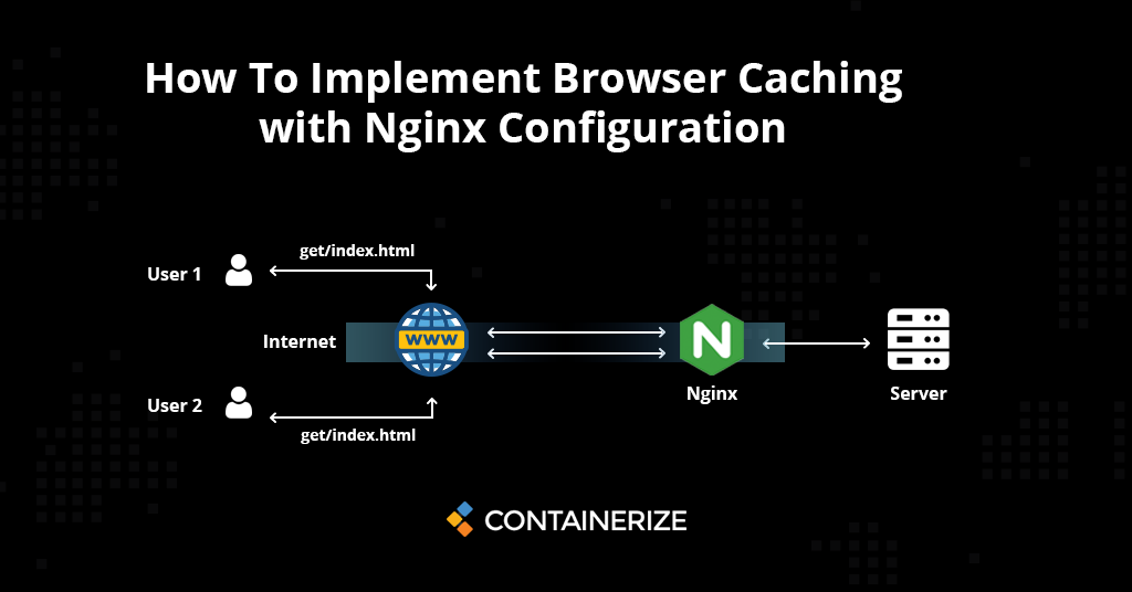
【Nginx负载均衡终极指南】:打造属于你的高效访问入口
.webp)
# 摘要
Nginx作为一款高性能的HTTP和反向代理服务器,已成为实现负载均衡的首选工具之一。本文首先介绍了Nginx负载均衡的概念及其理论基础,阐述了负载均衡的定义、作用以及常见算法,进而探讨了Nginx的架构和关键组件。文章深入到配置实践,解析了Nginx配置文件的关键指令,并通过具体配置案例展示了如何在不同场景下设置Nginx以实现高效的负载分配。
云计算助力餐饮业:系统部署与管理的最佳实践
# 摘要
云计算作为一种先进的信息技术,在餐饮业中的应用正日益普及。本文详细探讨了云计算与餐饮业务的结合方式,包括不同类型和部署模型的云服务,并分析了其在成本效益、扩展性、资源分配和高可用性等方面的优势。文中还提供餐饮业务系统云部署的实践案例,包括云服务选择、迁移策略以及安全合规性方面的考量。进一步地,文章深入讨论了餐饮业务云管理与优化的方法,并通过案例研究展示了云计算在餐饮业中的成功应用。最后,本文对云计算在餐饮业中
【Nginx安全与性能】:根目录迁移,如何在保障安全的同时优化性能
# 摘要
本文对Nginx根目录迁移过程、安全性加固策略、性能优化技巧及实践指南进行了全面的探讨。首先概述了根目录迁移的必要性与准备步骤,随后深入分析了如何加固Nginx的安全性,包括访问控制、证书加密、
RJ-CMS主题模板定制:个性化内容展示的终极指南

# 摘要
本文详细介绍了RJ-CMS主题模板定制的各个方面,涵盖基础架构、语言教程、最佳实践、理论与实践、高级技巧以及未来发展趋势。通过解析RJ-CMS模板的文件结构和继承机制,介绍基本语法和标签使用,本文旨在提供一套系统的方法论,以指导用户进行高效和安全的主题定制。同时,本文也探讨了如何优化定制化模板的性能,并分析了模板定制过程中的高级技术应用和安全性问题。最后,本文展望了RJ-CMS模板定制的
【板坯连铸热传导进阶】:专家教你如何精确预测和控制温度场

# 摘要
本文系统地探讨了板坯连铸过程中热传导的基础理论及其优化方法。首先,介绍了热传导的基本理论和建立热传导模型的方法,包括导热微分方程及其边界和初始条件的设定。接着,详细阐述了热传导模型的数值解法,并分析了影响模型准确性的多种因素,如材料热物性、几何尺寸和环境条件。本文还讨论了温度场预测的计算方法,包括有限差分法、有限元法和边界元法,并对温度场控制技术进行了深入分析。最后,文章探讨了温度场优化策略、
【性能优化大揭秘】:3个方法显著提升Android自定义View公交轨迹图响应速度

# 摘要
本文旨在探讨Android自定义View在实现公交轨迹图时的性能优化。首先介绍了自定义View的基础知识及其在公交轨迹图中应用的基本要求。随后,文章深入分析了性能瓶颈,包括常见性能问题如界面卡顿、内存泄漏,以及绘制过程中的性能考量。接着,提出了提升响应速度的三大方法论,包括减少视图层次、视图更新优化以及异步处理和多线程技术应用。第四章通过实践应用展示了性能优化的实战过程和
Python环境管理:一次性解决Scripts文件夹不出现的根本原因

# 摘要
本文系统地探讨了Python环境的管理,从Python安装与配置的基础知识,到Scripts文件夹生成和管理的机制,再到解决环境问题的实践案例。文章首先介绍了Python环境管理的基本概念,详细阐述了安装Python解释器、配置环境变量以及使用虚拟环境的重要性。随
通讯录备份系统高可用性设计:MySQL集群与负载均衡实战技巧

# 摘要
本文探讨了通讯录备份系统的高可用性架构设计及其实际应用。首先对MySQL集群基础进行了详细的分析,包括集群的原理、搭建与配置以及数据同步与管理。随后,文章深入探讨了负载均衡技术的原理与实践,及其与MySQL集群的整合方法。在此基础上,详细阐述了通讯录备份系统的高可用性架构设计,包括架构的需求与目标、双活或多活数据库架构的构建,以及监
【20分钟精通MPU-9250】:九轴传感器全攻略,从入门到精通(必备手册)

# 摘要
本文对MPU-9250传感器进行了全面的概述,涵盖了其市场定位、理论基础、硬件连接、实践应用、高级应用技巧以及故障排除与调试等方面。首先,介绍了MPU-9250作为一种九轴传感器的工作原理及其在数据融合中的应用。随后,详细阐述了传感器的硬件连
资源上传下载、课程学习等过程中有任何疑问或建议,欢迎提出宝贵意见哦~我们会及时处理!
点击此处反馈


专栏目录
最低0.47元/天 解锁专栏
买1年送3月
百万级
高质量VIP文章无限畅学
千万级
优质资源任意下载
C知道
免费提问 ( 生成式Al产品 )