【线性时间排序算法详解】：揭秘快速排序与堆排序的实战应用，提升代码效率

# 1. 排序算法概述

排序算法是计算机科学中至关重要的算法，用于对数据进行组织和排列。它们在各种应用中发挥着关键作用，从数据分析到机器学习。排序算法的种类繁多，每种算法都有其独特的优点和缺点。本章将提供排序算法的概述，介绍其基本概念和分类。

排序算法可以分为两大类：基于比较的排序和非基于比较的排序。基于比较的排序通过比较元素之间的值来确定它们的顺序，而非基于比较的排序则使用其他方法，例如元素的键值或哈希函数。本章将重点介绍基于比较的排序算法，包括快速排序和堆排序。

# 2. 快速排序理论与实践

### 2.1 快速排序算法原理

#### 2.1.1 分治思想与递归实现

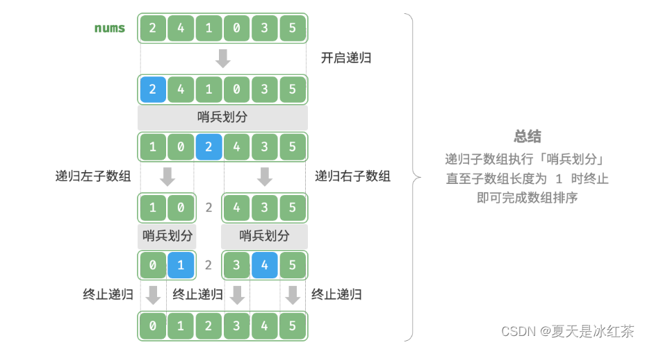
快速排序算法遵循分治思想，将一个无序数组划分为两个子数组：一个包含所有小于或等于枢轴元素的元素，另一个包含所有大于枢轴元素的元素。然后递归地对这两个子数组应用相同的过程，直到每个子数组只有一个元素或为空。

graph LR
subgraph 快速排序
    A[0, n-1] --> B[0, p-1]
    A[0, n-1] --> C[p, n-1]
    B[0, p-1] --> D[0, p-1]
    C[p, n-1] --> E[p, n-1]
    D[0, p-1] --> A[0, p-1]
    E[p, n-1] --> A[p, n-1]
end

**递归实现：**

def quick_sort(array, left, right):
    if left < right:
        pivot = partition(array, left, right)
        quick_sort(array, left, pivot - 1)
        quick_sort(array, pivot + 1, right)

#### 2.1.2 枢轴元素的选择与分区

枢轴元素的选择对于快速排序的性能至关重要。一个好的枢轴元素可以将数组大致分成大小相等的两个子数组，从而提高递归的效率。

**分区过程：**

def partition(array, left, right):
    pivot = array[right]
    i = left - 1
    for j in range(left, right):
        if array[j] <= pivot:
            i += 1
            array[i], array[j] = array[j], array[i]
    array[i + 1], array[right] = array[right], array[i + 1]
    return i + 1

### 2.2 快速排序代码实现

#### 2.2.1 C语言实现

#include <stdio.h>
#include <stdlib.h>

void quick_sort(int *array, int left, int right) {
    if (left < right) {
        int pivot = partition(array, left, right);
        quick_sort(array, left, pivot - 1);
        quick_sort(array, pivot + 1, right);
    }
}

int partition(int *array, int left, int right) {
    int pivot = array[right];
    int i = left - 1;
    for (int j = left; j < right; j++) {
        if (array[j] <= pivot) {
            i++;
            int temp = array[i];
            array[i] = array[j];
            array[j] = temp;
        }
    }
    int temp = array[i + 1];
    array[i + 1] = array[right];
    array[right] = temp;
    return i + 1;
}

int main() {
    int array[] = {10, 7, 8, 9, 1, 5};
    int n = sizeof(array) / sizeof(array[0]);
    quick_sort(array, 0, n - 1);
    for (int i = 0; i < n; i++) {
        printf("%d ", array[i]);
    }
    printf("\n");
    return 0;
}

#### 2.2.2 Python实现

def quick_sort(array, left, right):
    if left < right:
        pivot = partition(array, left, right)
        quick_sort(array, left, pivot - 1)
        quick_sort(array, pivot + 1, right)

def partition(array, left, right):
    pivot = array[right]
    i = left - 1
    for j in range(left, right):
        if array[j] <= pivot:
            i += 1
            array[i], array[j] = array[j], array[i]
    array[i + 1], array[right] = array[right], array[i + 1]
    return i + 1

array = [10, 7, 8, 9, 1, 5]
quick_sort(array, 0, len(array) - 1)
print(array)

### 2.3 快速排序性能分析

#### 2.3.1 时间复杂度

快速排序的平均时间复杂度为 O(n log n)，其中 n 是数组的长度。然而，在最坏的情况下，当数组已经有序或逆序时，时间复杂度退化为 O(n^2)。

#### 2.3.2 空间复杂度

快速排序的空间复杂度为 O(log n)，因为递归调用栈的深度不会超过数组的深度。

# 3. 堆排序理论与实践

### 3.1 堆排序算法原理

#### 3.1.1 堆数据结构

堆是一种完全二叉树，其中每个节点的值都大于或等于其子节点的值。堆有两种类型：最大堆和最小堆。在最大堆中，根节点的值是堆中最大的值，而在最小堆中，根节点的值是堆中最小的值。

#### 3.1.2 堆排序过程

堆排序算法通过将输入数组转换为最大堆，然后依次弹出堆顶元素并将其插入到数组的末尾来实现排序。堆排序过程分为以下步骤：

1. **建堆：**将输入数组转换为最大堆。
2. **弹出堆顶：**弹出堆顶元素并将其插入到数组的末尾。
3. **调整堆：**将剩余的堆调整为最大堆。
4. **重复步骤 2 和 3：**重复步骤 2 和 3，直到堆为空。

### 3.2 堆排序代码实现

#### 3.2.1 C++实现

void heapSort(int arr[], int n) {
    // 建堆
    for (int i = n / 2 - 1; i >= 0; i--) {
        heapify(arr, n, i);
    }

    // 依次弹出堆顶元素并插入到数组末尾
    for (int i = n - 1; i >= 0; i--) {
        // 交换堆顶元素和数组末尾元素
        int temp = arr[0];
        arr[0] = arr[i];
        arr[i] = temp;

        // 调整剩余的堆
        heapify(arr, i, 0);
    }
}

void heapify(int arr[], int n, int i) {
    int largest = i;
    int left = 2 * i + 1;
    int right = 2 * i + 2;

    // 找出左子节点和右子节点中较大的那个
    if (left < n && arr[left] > arr[largest]) {
        largest = left;
    }
    if (right < n && arr[right] > arr[largest]) {
        largest = right;
    }

    // 如果最大的不是根节点，则交换根节点和最大的子节点
    if (largest != i) {
        int temp = arr[i];
        arr[i] = arr[largest];
        arr[largest] = temp;

        // 递归调整子堆
        heapify(arr, n, largest);
    }
}

#### 3.2.2 Java实现

public class HeapSort {

    public static void heapSort(int[] arr) {
        // 建堆
        for (int i = arr.length / 2 - 1; i >= 0; i--) {
            heapify(arr, i, arr.length);
        }

        // 依次弹出堆顶元素并插入到数组末尾
        for (int i = arr.length - 1; i >= 0; i--) {
            // 交换堆顶元素和数组末尾元素
            int temp = arr[0];
            arr[0] = arr[i];
            arr[i] = temp;

            // 调整剩余的堆
            heapify(arr, 0, i);
        }
    }

    private static void heapify(int[] arr, int i, int n) {
        int largest = i;
        int left = 2 * i + 1;
        int right = 2 * i + 2;

        // 找出左子节点和右子节点中较大的那个
        if (left < n && arr[left] > arr[largest]) {
            largest = left;
        }
        if (right < n && arr[right] > arr[largest]) {
            largest = right;
        }

        // 如果最大的不是根节点，则交换根节点和最大的子节点
        if (largest != i) {
            int temp = arr[i];
            arr[i] = arr[largest];
            arr[largest] = temp;

            // 递归调整子堆
            heapify(arr, largest, n);
        }
    }
}

### 3.3 堆排序性能分析

#### 3.3.1 时间复杂度

堆排序的时间复杂度为 O(n log n)，其中 n 是数组的长度。

#### 3.3.2 空间复杂度

堆排序的空间复杂度为 O(1)，因为它不需要额外的空间来存储辅助数据结构。

# 4. 快速排序与堆排序对比

### 4.1 算法原理对比

#### 4.1.1 分治与堆排序

快速排序采用分治思想，将待排序数组划分为两个子数组，分别递归排序子数组，最后合并子数组得到有序数组。

堆排序则采用堆数据结构，将待排序数组构建成一个大顶堆，不断从堆顶取出最大元素，插入到有序数组中，直到堆为空。

#### 4.1.2 枢轴元素选择与堆顶元素

快速排序中，枢轴元素的选择对排序效率至关重要。一般情况下，选择数组中位数或随机元素作为枢轴元素。

堆排序中，堆顶元素始终是当前堆中最大的元素。

### 4.2 性能对比

#### 4.2.1 时间复杂度分析

快速排序的时间复杂度为 O(n log n) 在平均情况下，但最坏情况下为 O(n^2)。

堆排序的时间复杂度始终为 O(n log n)。

| 算法 | 平均时间复杂度 | 最坏时间复杂度 |
|---|---|---|
| 快速排序 | O(n log n) | O(n^2) |
| 堆排序 | O(n log n) | O(n log n) |

#### 4.2.2 空间复杂度分析

快速排序的空间复杂度为 O(log n)，因为它使用递归调用。

堆排序的空间复杂度为 O(1)，因为它不需要额外的空间。

| 算法 | 空间复杂度 |
|---|---|
| 快速排序 | O(log n) |
| 堆排序 | O(1) |

### 4.3 应用场景对比

#### 4.3.1 快速排序适用场景

* 数据量较小或中等
* 数据分布相对均匀
* 需要快速排序结果

#### 4.3.2 堆排序适用场景

* 数据量较大
* 数据分布不均匀
* 需要稳定排序（即相同元素保持相对顺序）
* 需要在排序过程中进行其他操作（如查找最大值）

**代码示例：**

# 快速排序
def quick_sort(arr):
    if len(arr) <= 1:
        return arr

    pivot = arr[len(arr) // 2]
    left = [x for x in arr if x < pivot]
    middle = [x for x in arr if x == pivot]
    right = [x for x in arr if x > pivot]

    return quick_sort(left) + middle + quick_sort(right)

# 堆排序
def heap_sort(arr):
    def heapify(arr, n, i):
        largest = i
        left = 2 * i + 1
        right = 2 * i + 2

        if left < n and arr[left] > arr[largest]:
            largest = left

        if right < n and arr[right] > arr[largest]:
            largest = right

        if largest != i:
            arr[i], arr[largest] = arr[largest], arr[i]
            heapify(arr, n, largest)

    n = len(arr)

    # 构建大顶堆
    for i in range(n // 2 - 1, -1, -1):
        heapify(arr, n, i)

    # 排序
    for i in range(n - 1, 0, -1):
        arr[i], arr[0] = arr[0], arr[i]
        heapify(arr, i, 0)

    return arr

**表格：快速排序与堆排序对比**

| 特征 | 快速排序 | 堆排序 |
|---|---|---|
| 时间复杂度 | 平均 O(n log n)，最坏 O(n^2) | O(n log n) |
| 空间复杂度 | O(log n) | O(1) |
| 稳定性 | 不稳定 | 稳定 |
| 适用场景 | 数据量较小或中等，数据分布均匀 | 数据量较大，数据分布不均匀，需要稳定排序 |

# 5. 排序算法在实战中的应用

排序算法在实际应用中发挥着至关重要的作用，广泛应用于数据预处理、机器学习和分布式大数据处理等领域。

### 5.1 数据预处理中的排序

#### 5.1.1 数据清洗与排序

数据清洗是数据预处理的重要步骤，旨在去除数据中的异常值和噪声。排序算法可以用于识别异常值，例如：

import numpy as np

# 原始数据
data = [1, 3, 5, 7, 9, 11, 13, 15, 17, 19, 21, 23, 25, 27, 29, 31, 33, 35, 37, 39]

# 排序数据
sorted_data = np.sort(data)

# 识别异常值（大于平均值3个标准差）
mean = np.mean(sorted_data)
std = np.std(sorted_data)
threshold = mean + 3 * std
outliers = [x for x in sorted_data if x > threshold]

print("异常值：", outliers)

#### 5.1.2 数据归一化与排序

数据归一化是将数据映射到特定范围的过程，以消除不同特征之间的量纲差异。排序算法可以用于对数据进行归一化，例如：

# 原始数据
data = [1, 3, 5, 7, 9, 11, 13, 15, 17, 19, 21, 23, 25, 27, 29, 31, 33, 35, 37, 39]

# 排序数据
sorted_data = np.sort(data)

# 最大-最小归一化
normalized_data = (sorted_data - np.min(sorted_data)) / (np.max(sorted_data) - np.min(sorted_data))

print("归一化数据：", normalized_data)

### 5.2 机器学习中的排序

#### 5.2.1 特征选择与排序

特征选择是机器学习中识别和选择最相关特征的过程。排序算法可以用于对特征进行排序，例如：

import pandas as pd
from sklearn.feature_selection import SelectKBest, chi2

# 原始数据
data = pd.DataFrame({
    "feature1": [1, 3, 5, 7, 9, 11, 13, 15, 17, 19, 21, 23, 25, 27, 29, 31, 33, 35, 37, 39],
    "feature2": [2, 4, 6, 8, 10, 12, 14, 16, 18, 20, 22, 24, 26, 28, 30, 32, 34, 36, 38, 40],
    "target": [0, 1, 0, 1, 0, 1, 0, 1, 0, 1, 0, 1, 0, 1, 0, 1, 0, 1, 0, 1]
})

# 使用卡方检验对特征进行排序
selector = SelectKBest(chi2, k=2)
selector.fit(data[["feature1", "feature2"]], data["target"])

# 排序后的特征
sorted_features = selector.get_support(indices=True)
print("排序后的特征：", sorted_features)

#### 5.2.2 模型训练与排序

模型训练是机器学习中根据训练数据学习模型的过程。排序算法可以用于对模型进行排序，例如：

import numpy as np
from sklearn.model_selection import cross_val_score

# 原始数据
data = pd.DataFrame({
    "feature1": [1, 3, 5, 7, 9, 11, 13, 15, 17, 19, 21, 23, 25, 27, 29, 31, 33, 35, 37, 39],
    "feature2": [2, 4, 6, 8, 10, 12, 14, 16, 18, 20, 22, 24, 26, 28, 30, 32, 34, 36, 38, 40],
    "target": [0, 1, 0, 1, 0, 1, 0, 1, 0, 1, 0, 1, 0, 1, 0, 1, 0, 1, 0, 1]
})

# 不同模型
models = [
    LinearRegression(),
    LogisticRegression(),
    DecisionTreeClassifier(),
    RandomForestClassifier()
]

# 使用交叉验证对模型进行排序
scores = []
for model in models:
    score = cross_val_score(model, data[["feature1", "feature2"]], data["target"], cv=5).mean()
    scores.append(score)

# 排序后的模型
sorted_models = np.argsort(scores)[::-1]
print("排序后的模型：", sorted_models)

### 5.3 大数据处理中的排序

#### 5.3.1 分布式排序技术

分布式排序技术将大数据集分解成较小的块，并在多个节点上并行处理。排序算法在分布式环境中可以有效利用计算资源，例如：

graph LR
    subgraph 分布式排序
        A[Map] --> B[Shuffle] --> C[Sort] --> D[Reduce]
    end

#### 5.3.2 云计算平台中的排序

云计算平台提供预先配置的排序服务，可以简化大数据集的排序过程。例如：

# 使用 AWS EMR 运行 Spark 排序作业
spark_session = SparkSession.builder \
    .master("yarn") \
    .appName("Spark Sort") \
    .getOrCreate()

data = spark_session.read.csv("s3://my-bucket/data.csv")
sorted_data = data.sort("column_name")
sorted_data.write.csv("s3://my-bucket/sorted_data.csv")