aero bike bird boat bottle bus car cat chair cow table dog horse mbike person plant sheep sofa train tv
Our rank 3 1 2 1 1 2 2 4 1 1 1 4 2 2 1 1 2 1 4 1
Our score .180 .411 .092 .098 .249 .349 .396 .110 .155 .165 .110 .062 .301 .337 .267 .140 .141 .156 .206 .336
Darmstadt .301
INRIA Normal .092 .246 .012 .002 .068 .197 .265 .018 .097 .039 .017 .016 .225 .153 .121 .093 .002 .102 .157 .242
INRIA Plus .136 .287 .041 .025 .077 .279 .294 .132 .106 .127 .067 .071 .335 .249 .092 .072 .011 .092 .242 .275
IRISA .281 .318 .026 .097 .119 .289 .227 .221 .175 .253
MPI Center .060 .110 .028 .031 .000 .164 .172 .208 .002 .044 .049 .141 .198 .170 .091 .004 .091 .034 .237 .051
MPI ESSOL .152 .157 .098 .016 .001 .186 .120 .240 .007 .061 .098 .162 .034 .208 .117 .002 .046 .147 .110 .054
Oxford .262 .409 .393 .432 .375 .334
TKK .186 .078 .043 .072 .002 .116 .184 .050 .028 .100 .086 .126 .186 .135 .061 .019 .036 .058 .067 .090
Table 1. PASCAL VOC 2007 results. Average precision scores of our system and other systems that entered the competition [7]. Empty
boxes indicate that a method was not tested in the corresponding class. The best score in each class is shown in bold. Our current system
ranks first in 10 out of 20 classes. A preliminary version of our system ranked first in 6 classes in the official competition.
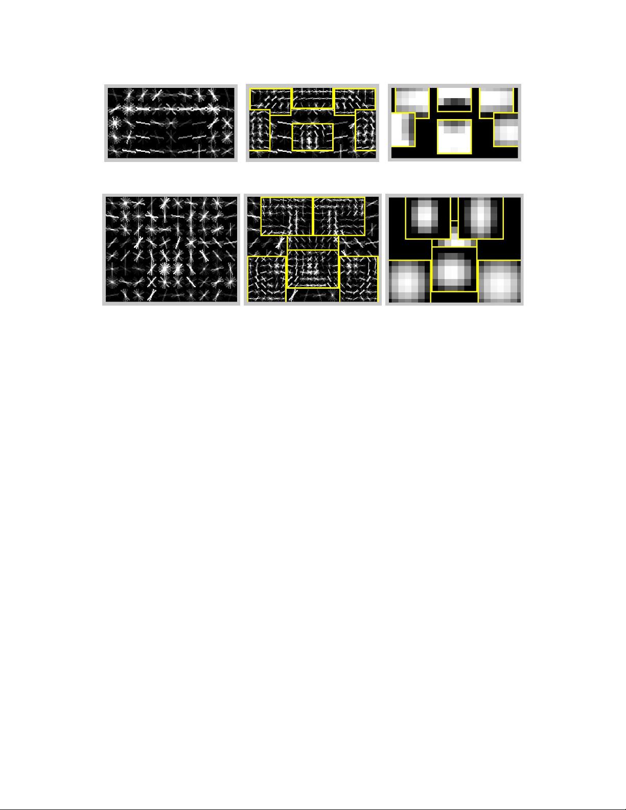
Bottle
Car
Bicycle
Sofa
Figure 4. Some models learned from the PASCAL VOC 2007 dataset. We show the total energy in each orientation of the HOG cells in
the root and part filters, with the part filters placed at the center of the allowable displacements. We also show the spatial model for each
part, where bright values represent “cheap” placements, and dark values represent “expensive” placements.
in the PASCAL competition was .16, obtained using a rigid
template model of HOG features [5]. The best previous re-
sult of .19 adds a segmentation-based verification step [20].
Figure 6 summarizes the performance of several models we
trained. Our root-only model is equivalent to the model
from [5] and it scores slightly higher at .18. Performance
jumps to .24 when the model is trained with a LSVM that
selects a latent position and scale for each positive example.
This suggests LSVMs are useful even for rigid templates
because they allow for self-adjustment of the detection win-
dow in the training examples. Adding deformable parts in-
creases performance to .34 AP — a factor of two above the
best previous score. Finally, we trained a model with parts
but no root filter and obtained .29 AP. This illustrates the
advantage of using a multiscale representation.
We also investigated the effect of the spatial model and
allowable deformations on the 2006 person dataset. Recall
that s
i
is the allowable displacement of a part, measured in
HOG cells. We trained a rigid model with high-resolution
parts by setting s
i
to 0. This model outperforms the root-
only system by .27 to .24. If we increase the amount of
allowable displacements without using a deformation cost,
we start to approach a bag-of-features. Performance peaks
at s
i
=1, suggesting it is useful to constrain the part dis-
placements. The optimal strategy allows for larger displace-
ments while using an explicit deformation cost. The follow-
6
aero bike bird boat bottle bus car cat chair cow table dog horse mbike person plant sheep sofa train tv
Our rank 3 1 2 1 1 2 2 4 1 1 1 4 2 2 1 1 2 1 4 1
Our score .180 .411 .092 .098 .249 .349 .396 .110 .155 .165 .110 .062 .301 .337 .267 .140 .141 .156 .206 .336
Darmstadt .301
INRIA Normal .092 .246 .012 .002 .068 .197 .265 .018 .097 .039 .017 .016 .225 .153 .121 .093 .002 .102 .157 .242
INRIA Plus .136 .287 .041 .025 .077 .279 .294 .132 .106 .127 .067 .071 .335 .249 .092 .072 .011 .092 .242 .275
IRISA .281 .318 .026 .097 .119 .289 .227 .221 .175 .253
MPI Center .060 .110 .028 .031 .000 .164 .172 .208 .002 .044 .049 .141 .198 .170 .091 .004 .091 .034 .237 .051
MPI ESSOL .152 .157 .098 .016 .001 .186 .120 .240 .007 .061 .098 .162 .034 .208 .117 .002 .046 .147 .110 .054
Oxford .262 .409 .393 .432 .375 .334
TKK .186 .078 .043 .072 .002 .116 .184 .050 .028 .100 .086 .126 .186 .135 .061 .019 .036 .058 .067 .090
Table 1. PASCAL VOC 2007 results. Average precision scores of our system and other systems that entered the competition [7]. Empty
boxes indicate that a method was not tested in the corresponding class. The best score in each class is shown in bold. Our current system
ranks first in 10 out of 20 classes. A preliminary version of our system ranked first in 6 classes in the official competition.
Bottle
Car
Bicycle
Sofa
Figure 4. Some models learned from the PASCAL VOC 2007 dataset. We show the total energy in each orientation of the HOG cells in
the root and part filters, with the part filters placed at the center of the allowable displacements. We also show the spatial model for each
part, where bright values represent “cheap” placements, and dark values represent “expensive” placements.
in the PASCAL competition was .16, obtained using a rigid
template model of HOG features [5]. The best previous re-
sult of .19 adds a segmentation-based verification step [20].
Figure 6 summarizes the performance of several models we
trained. Our root-only model is equivalent to the model
from [5] and it scores slightly higher at .18. Performance
jumps to .24 when the model is trained with a LSVM that
selects a latent position and scale for each positive example.
This suggests LSVMs are useful even for rigid templates
because they allow for self-adjustment of the detection win-
dow in the training examples. Adding deformable parts in-
creases performance to .34 AP — a factor of two above the
best previous score. Finally, we trained a model with parts
but no root filter and obtained .29 AP. This illustrates the
advantage of using a multiscale representation.
We also investigated the effect of the spatial model and
allowable deformations on the 2006 person dataset. Recall
that s
i
is the allowable displacement of a part, measured in
HOG cells. We trained a rigid model with high-resolution
parts by setting s
i
to 0. This model outperforms the root-
only system by .27 to .24. If we increase the amount of
allowable displacements without using a deformation cost,
we start to approach a bag-of-features. Performance peaks
at s
i
=1, suggesting it is useful to constrain the part dis-
placements. The optimal strategy allows for larger displace-
ments while using an explicit deformation cost. The follow-
6
(a) car
aero bike bird boat bottle bus car cat chair cow table dog horse mbike person plant sheep sofa train tv
Our rank 3 1 2 1 1 2 2 4 1 1 1 4 2 2 1 1 2 1 4 1
Our score .180 .411 .092 .098 .249 .349 .396 .110 .155 .165 .110 .062 .301 .337 .267 .140 .141 .156 .206 .336
Darmstadt .301
INRIA Normal .092 .246 .012 .002 .068 .197 .265 .018 .097 .039 .017 .016 .225 .153 .121 .093 .002 .102 .157 .242
INRIA Plus .136 .287 .041 .025 .077 .279 .294 .132 .106 .127 .067 .071 .335 .249 .092 .072 .011 .092 .242 .275
IRISA .281 .318 .026 .097 .119 .289 .227 .221 .175 .253
MPI Center .060 .110 .028 .031 .000 .164 .172 .208 .002 .044 .049 .141 .198 .170 .091 .004 .091 .034 .237 .051
MPI ESSOL .152 .157 .098 .016 .001 .186 .120 .240 .007 .061 .098 .162 .034 .208 .117 .002 .046 .147 .110 .054
Oxford .262 .409 .393 .432 .375 .334
TKK .186 .078 .043 .072 .002 .116 .184 .050 .028 .100 .086 .126 .186 .135 .061 .019 .036 .058 .067 .090
Table 1. PASCAL VOC 2007 results. Average precision scores of our system and other systems that entered the competition [7]. Empty
boxes indicate that a method was not tested in the corresponding class. The best score in each class is shown in bold. Our current system
ranks first in 10 out of 20 classes. A preliminary version of our system ranked first in 6 classes in the official competition.
Figure 4. Some models learned from the PASCAL VOC 2007 dataset. We show the total energy in each orientation of the HOG cells in
the root and part filters, with the part filters placed at the center of the allowable displacements. We also show the spatial model for each
part, where bright values represent “cheap” placements, and dark values represent “expensive” placements.
in the PASCAL competition was .16, obtained using a rigid
template model of HOG features [5]. The best previous re-
sult of .19 adds a segmentation-based verification step [20].
Figure 6 summarizes the performance of several models we
trained. Our root-only model is equivalent to the model
from [5] and it scores slightly higher at .18. Performance
jumps to .24 when the model is trained with a LSVM that
selects a latent position and scale for each positive example.
This suggests LSVMs are useful even for rigid templates
because they allow for self-adjustment of the detection win-
dow in the training examples. Adding deformable parts in-
creases performance to .34 AP — a factor of two above the
best previous score. Finally, we trained a model with parts
but no root filter and obtained .29 AP. This illustrates the
advantage of using a multiscale representation.
We also investigated the effect of the spatial model and
allowable deformations on the 2006 person dataset. Recall
that s
i
is the allowable displacement of a part, measured in
HOG cells. We trained a rigid model with high-resolution
parts by setting s
i
to 0. This model outperforms the root-
only system by .27 to .24. If we increase the amount of
allowable displacements without using a deformation cost,
we start to approach a bag-of-features. Performance peaks
at s
i
= 1, suggesting it is useful to constrain the part dis-
placements. The optimal strategy allows for larger displace-
ments while using an explicit deformation cost. The follow-
6
(b) bicycle
Figure 1.2: Models with a single root filter. Images reproduced from [34].
In our formulation, we treat the subcategory labels as latent information, analogous to
the latent cluster labels used when fitting mixture models with expectation maximization
(EM). In contrast to existing approaches, such as EM, we use nonprobabilistic, discriminative
frameworks — latent SVM and weak-label structural SVM — to learn mixtures. Returning
to the bicycle example, our system automatically learns subcategories for: side, 45
◦
angle,
and front/rear views.
Latent orientation. For many object categories, photographs taken by people typically
capture category instances with significant variation in out-of-plane rotation. Empirically, we
find that our method for learning subcategories tends to cluster instances that have similar
out-of-plane rotations — modulo 180
◦
— together. In the horse category, for example, one
of the learned clusters corresponds to side views. Unfortunately this cluster includes both
left and right-facing horses, and because their appearance is represented jointly, the result
is a model ideally suited to detect two-headed horses (see Figure 1.3 top). To address this
problem, we enrich our models by treating orientation within a subcategory as a latent,
8


 我的内容管理
展开
我的内容管理
展开


