

SAS PROC MIXED 13
identifies the contrast in the table. A label is required for every contrast specified. Labels can be up to 20
characters and must be enclosed in single quotes.
fixed-effect
identifies an effect that appears in the MODEL statement. The keyword INTERCEPT can be used as an
effect when an intercept is fitted in the model. You do not need to include all effects that are in the
MODEL statement.
random-effect
identifies an effect that appears in the RANDOM statement. The first random effect must follow a vertical
bar (|); however, random effects do not have to be specified.
values
are constants that are elements of the L matrix associated with the fixed and random effects.
The rows of L' are specified in order and are separated by commas. The rows of the K' component of L' are
specified on the left side of the vertical bars (|). These rows test the fixed effects and are, therefore, checked for
estimability. The rows of the M' component of L' are specified on the right side of the vertical bars. They test the
random effects, and no estimability checking is necessary.
If PROC MIXED finds the fixed-effects portion of the specified contrast to be nonestimable (see the SINGULAR=
option), then it displays "Non-est" for the contrast entries.
The following CONTRAST statement reproduces the F-test for the effect A in the split-plot example (see Example
41.1):
contrast 'A broad'
A 1 -1 0 A*B .5 .5 -.5 -.5 0 0 ,
A 1 0 -1 A*B .5 .5 0 0 -.5 -.5 / df=6;
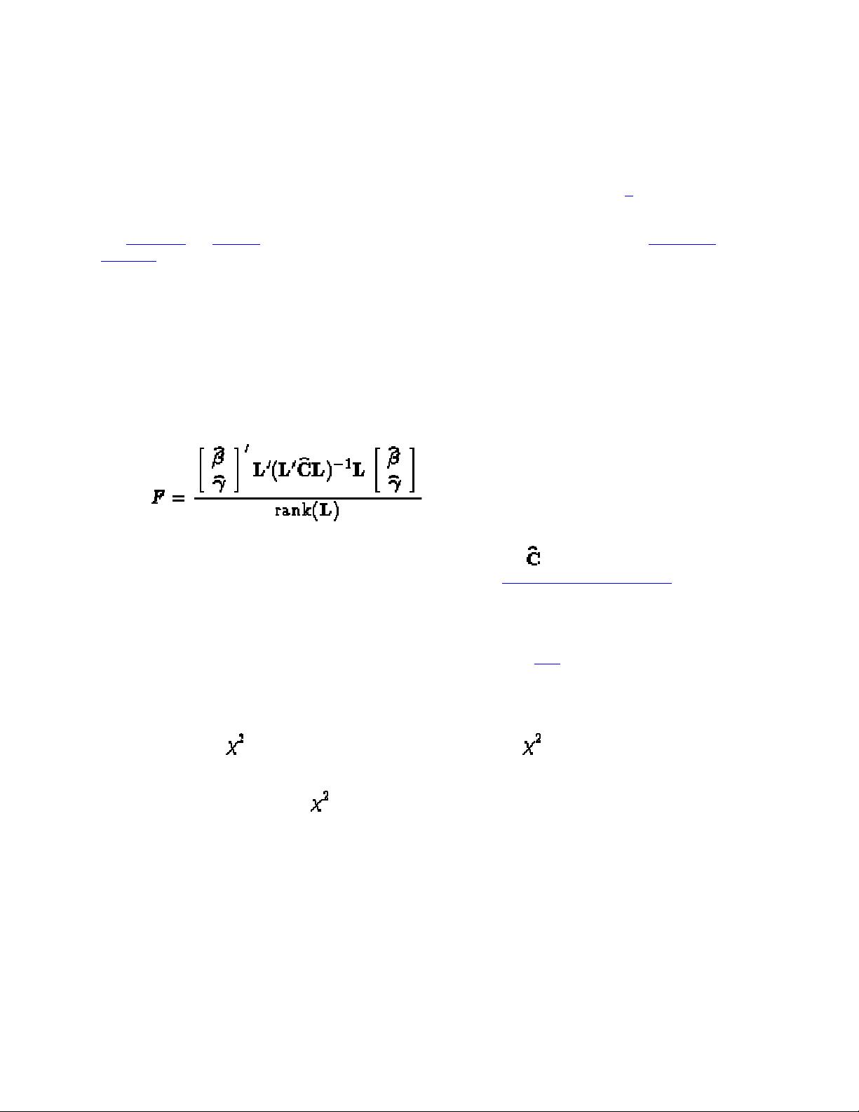
Note that no random effects are specified in the preceding contrast; thus, the inference space is broad. The resulting
F-test has two numerator degrees of freedom because L' has two rows. The denominator degrees of freedom is, by
default, the residual degrees of freedom (9), but the DF= option changes the denominator degrees of freedom to 6.
The following CONTRAST statement reproduces the F-test for A when Block and A*Block are considered fixed
effects (the narrow inference space):
contrast 'A narrow'
A 1 -1 0
A*B .5 .5 -.5 -.5 0 0 |
A*Block .25 .25 .25 .25
-.25 -.25 -.25 -.25
0 0 0 0 ,
A 1 0 -1
A*B .5 .5 0 0 -.5 -.5 |
A*Block .25 .25 .25 .25
0 0 0 0
-.25 -.25 -.25 -.25 ;
The preceding contrast does not contain coefficients for B and Block because they cancel out in estimated
differences between levels of A. Coefficients for B and Block are necessary when estimating the mean of one of the
levels of A in the narrow inference space (see Example 41.1
).
If the elements of L are not specified for an effect that contains a specified effect, then the elements of the specified
effect are automatically "filled in" over the levels of the higher-order effect. This feature is designed to preserve
estimability for cases when there are complex higher-order effects. The coefficients for the higher-order effect are
determined by equitably distributing the coefficients of the lower-level effect as in the construction of least squares
means. In addition, if the intercept is specified, it is distributed over all classification effects that are not contained
by any other specified effect. If an effect is not specified and does not contain any specified effects, then all of its

剩余79页未读,继续阅读

loveseeking
- 粉丝: 0
- 资源: 9
 我的内容管理
展开
我的内容管理
展开


最新资源
- Vue实现iOS原生Picker组件:详细解析与实现思路
- Arduino蓝牙小车:参数调试与功能控制
- 百度Java面试精华:200页精选资源涵盖核心知识点
- Swift使用CoreData填坑指南:CoreData在Swift 3.0的变化
- 微距离无线充电器创新设计及其实验探索
- MTK Android平台开发全攻略:44步详解流程
- RecyclerView全面解析:替代ListView的新选择
- Android开发:自动适配中英文键盘解决方案
- Android调用WebService接口教程
- Android开发:BitmapUtil图片处理全解析与实例
- Android多线程断点续传实现详解
- PCA算法在人脸识别会议签到系统中的应用
- EventBus 3.0:Android事件总线详解与实战应用
- Android FileUtil:全面解析文件操作实用技巧与实例
- RecyclerView添加头部和尾部实战教程
- Android实现微博滑动固定顶部栏实战与优化
资源上传下载、课程学习等过程中有任何疑问或建议,欢迎提出宝贵意见哦~我们会及时处理!
点击此处反馈


