
mean values of each calendar day, 2) fit a probability
distribution (such as the three-parameter gamma distri-
bution) to the daily anomalies for each Julian day, and
3) compute the thresholds from the fitted probability
distributions. Folland et al. (1999) also recommended
that data from additional proximate calendar days be
added to improve the stability of the probability distri-
bution parameter estimates but that those days should
be far enough apart such that data from different days
are effectively independent. This method was imple-
mented in Jones et al. (1999), who used five observa-
tions with 5-day intervals between them (referred to as
the 5SD window hereafter). In many other applications
(e.g., Frich et al. 2002; Klein Tank and Können 2003;
Kiktev et al. 2003), thresholds have been estimated us-
ing data from five consecutive days centered on the day
of interest (referred to as 5CD). In either case, the daily
thresholds are, in effect, percentiles estimated from
samples of no more than 5 ⫻ 30 ⫽ 150 days of data
when a standard 30-yr base period is used.
Despite the importance of these indicators in the de-
tection and monitoring of climate change, their statis-
tical properties have not been well documented. For
example, what differences would result in the index
time series when 5CD and 5SD windows are used?
Does the fact that the thresholds are “adapted” to (cal-
culated from) the base period cause any systematic dif-
ferences between the statistical properties of the index
time series during the base period (in base) and before
or after the base period (out of base)? Such differences
need to be understood before the indices can be used
with confidence for the purpose of climate change de-
tection and monitoring.
The main objective of this paper is to examine,
through Monte Carlo simulations, the characteristics of
the index time series that are obtained when threshold
functions are estimated with existing methods. We
show that these threshold estimation methods produce
substantial inhomogeneities in the index time series at
the beginning and end of the base period in the sense
that inhomogeneities become clearly apparent when a
large number of station series are averaged (Fig. 1) as
might be done in a climate change detection study. We
propose an approach that corrects the problem. The
remainder of this paper is organized as follows. We
describe existing methods for calculating thresholds
and index time series in section 2. The Monte Carlo
experiment that is used to study the performance of
these methods is also described in this section. Results
are presented in section 3. An improved method for
calculating the index time series is described and evalu-
ated in section 4. Conclusions and discussion follow in
section 5.
2. Methods
a. Threshold function estimation
There are three aspects to consider in constructing an
estimate of the threshold function. The first consider-
ation is the choice of base period. To ensure that index
time series can be easily extended into the future, the
base period is usually chosen to be consistent with a
recent World Meteorological Organisation (WMO) op-
erational climatology base period (e.g., 1961–90 or
1971–2000). Most studies have used the 1961–90 base
period because most indices of climate extremes were
developed in the late 1990s (Karl et al. 1999) and be-
cause there is greater availability of data during this
period than during other operational climatology base
periods.
The second consideration is the type of subsampling
that is used to select the data within the base period
that will be used for threshold estimation. In this study,
we use both the 5CD and 5SD windows. For example,
to estimate the threshold for 13 January, the 5CD win-
dow selects data for all days in the base period dated
11–15 January. In contrast, all base period observations
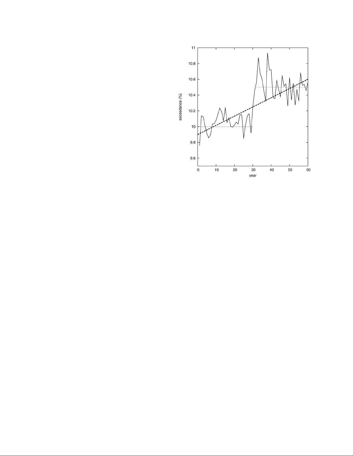
FIG. 1. Average of exceedance rate of daily values greater than
the 90th percentile in 1000 simulations in which the lag 1-day
autocorrelation has been set to 0.8. Thresholds are estimated us-
ing data from a 5-consecutive-day moving window and the em-
pirical quantile as defined in the text. The first 30 yr are used as
the base period. A jump (increase) in the exceedance rate is ap-
parent at the boundary between the in-base and out-of-base pe-
riods, as indicated by 30-yr averages (thin dashed lines). Because
of this jump, a highly significant trend (thick dashed line) can be
identified if a linear trend is fitted to the exceedance time series,
even though there is no trend in the simulated data.
1642 JOURNAL OF CLIMATE VOLUME 18
剩余11页未读,继续阅读

weixin_43492245
- 粉丝: 0
- 资源: 1
 我的内容管理
展开
我的内容管理
展开


最新资源
- C++标准程序库:权威指南
- Java解惑:奇数判断误区与改进方法
- C++编程必读:20种设计模式详解与实战
- LM3S8962微控制器数据手册
- 51单片机C语言实战教程:从入门到精通
- Spring3.0权威指南:JavaEE6实战
- Win32多线程程序设计详解
- Lucene2.9.1开发全攻略:从环境配置到索引创建
- 内存虚拟硬盘技术:提升电脑速度的秘密武器
- Java操作数据库:保存与显示图片到数据库及页面
- ISO14001:2004环境管理体系要求详解
- ShopExV4.8二次开发详解
- 企业形象与产品推广一站式网站建设技术方案揭秘
- Shopex二次开发:触发器与控制器重定向技术详解
- FPGA开发实战指南:创新设计与进阶技巧
- ShopExV4.8二次开发入门:解决升级问题与功能扩展
资源上传下载、课程学习等过程中有任何疑问或建议,欢迎提出宝贵意见哦~我们会及时处理!
点击此处反馈


