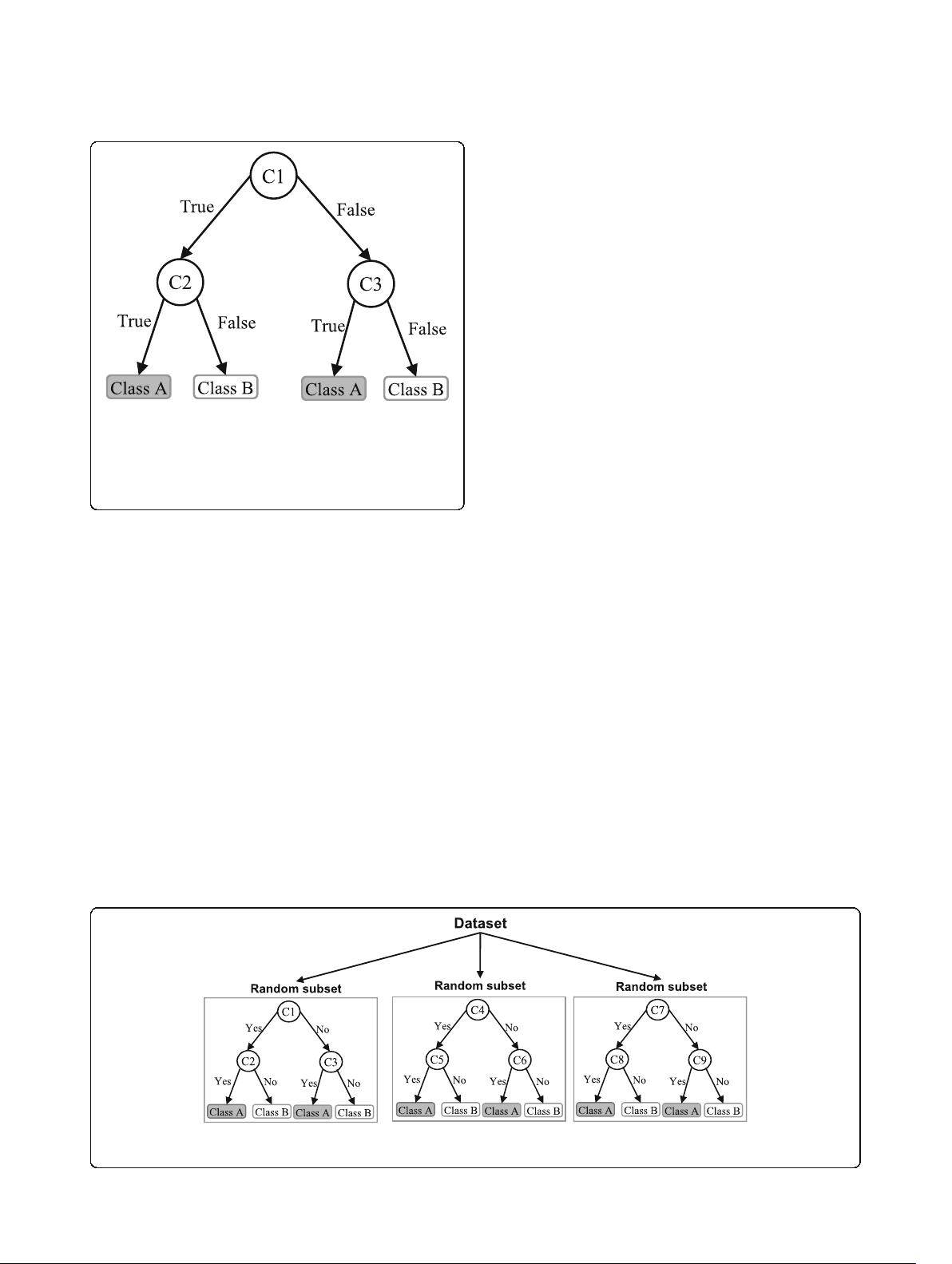
outcomeforasmallchangeintheinputdata.They
are very s ensitive to their training data, which makes
them error-prone to the test dataset. The different
DTs of a n RF are trained using the different parts of
the training dataset. To classify a new sample, the
input vector of that sample is required to pass down
with each DT of the forest. Each DT then considers
a different part of that input vector and gives a clas-
sification outcome. The forest then chooses the clas-
sification of having the most ‘ votes’ (for discrete
classification outcome) or the average of all trees in
the forest (for numeric classification outcome). Since
the R F algorithm considers the outcomes from many
different DTs, it can reduce the variance resulted
from the consideration of a single DT for the same
dataset. Figure 4 shows an illustration of the RF
algorithm.
Naïve Bayes
Naïve Bayes (NB) is a classification technique based on
the Bayes’ theorem [27]. This theorem can describe the
probability of an event based on the prior knowledge of
conditions related to that event. This classifier assumes
that a particular feature in a class is not directly related
to any other feature although features for that class
could have interdependence among themselves [28]. By
considering the task of classifying a new object (white
circle) to ei ther ‘ green’ class or ‘ red’ class, Fig. 5 pro-
vides an illustration about how the NB technique
works. According to this figure, it is reasonable to be-
lieve that any new object is twice as likely to have
‘green’ membership rather than ‘ red’ since there are
twice as many ‘green’ objects (40) as ‘red’.Inthe
Bayesian analysis, this belief is known as the prior
probability. Therefore, the prior probabilities of
‘green’ and ‘red’ are 0.67 (40 ÷ 60) and 0.33 (20 ÷
60), respectively. Now to classify the ‘ white’ object,
we need to draw a circle around this object which
encompasses several points (to be chosen prior) irre-
spective of their class labels. Four points (three ‘red’
and one ‘green) were considered in this figure. Thus,
the likelihood of ‘ white’ given ‘green’ is 0.025 (1 ÷ 40)
and the likelihood of ‘ white’ given ‘ red’ is 0.15 (3 ÷
20). Although the prior probability indicates that the
new ‘white’ object is more likely to have ‘ green’ mem-
bership, the likelihood shows that it is more likely to
be in the ‘red’ class. In the Bay esian analysis, the final
classifier is produced by c ombining both sources of
information (i.e., prior probability and likelihood
value). The ‘
multiplication’ function is used to com-
bine these two types o f information and the product
is called the ‘posterior’ probability. Finally, the poster-
ior probability of ‘ white’ being ‘green’ is 0.017 (0.67 ×
0.025) a nd the posterior probability of ‘ white’ being
‘red’ is 0.049 (0.33 × 0.15). Thus, the new ‘white’ ob-
ject should be classified as a member of the ‘red’ class
according to the NB technique.
Fig. 3 An illustration of a Decision tree. Each variable (C1, C2, and
C3) is represented by a circle and the decision outcomes (Class A
and Class B) are shown by rectangles. In order to successfully classify
a sample to a class, each branch is labelled with either ‘True’ or
‘False’ based on the outcome value from the test of its
ancestor node
Fig. 4 An illustration of a Random forest which consists of three different decision trees. Each of those three decision trees was trained using a
random subset of the training data
Uddin et al. BMC Medical Informatics and Decision Making (2019) 19:281 Page 4 of 16


