ode45 Solving Differential Equations: 10 Practical Tips to Help You Easily Solve Complex Problems
发布时间: 2024-09-15 05:48:50 阅读量: 36 订阅数: 40 
# ode45 Solving Differential Equations: 10 Practical Tips for Easy Problem-Solving
## 1. Fundamental Principles of ode45 Solver
The ode45 solver is a numerical method for solving ordinary differential equation systems, which uses the Runge-Kutta method. This method converts differential equations into a set of algebraic equations and then uses an iterative method to solve these equations to approximate the solution of the differential equations.
The ode45 solver offers a variety of solving options, including:
- **Solving Step Size:** Controls the step size the solver takes in each iteration. A smaller step size usually leads to a more accurate solution but also increases the computation time.
- **Tolerance:** Specifies the maximum error the solver allows during iteration. Smaller tolerance usually leads to a more accurate solution but also increases the computation time.
## 2. Optimizing Solving Performance
In practical applications, the ode45 solver may have issues with low efficiency and insufficient accuracy. To optimize solving performance, some techniques need to be mastered.
### 2.1 Adjusting Step Size and Tolerance
The ode45 solver employs adaptive step size control to solve differential equations. The size of the step size directly affects the accuracy and efficiency of the solution. Too large a step size reduces the accuracy of the solution; too small a step size reduces the efficiency of the solution.
You can adjust the step size and tolerance by setting the `RelTol` and `AbsTol` parameters in the solving options. `RelTol` specifies the relative error tolerance, and `AbsTol` specifies the absolute error tolerance.
```
options = odeset('RelTol', 1e-3, 'AbsTol', 1e-6);
[t, y] = ode45(@myfun, tspan, y0, options);
```
### 2.2 Selecting the Appropriate Solving Method
The ode45 solver offers various solving methods, including explicit and implicit methods. Explicit methods are faster but less stable; implicit methods are slower but more stable.
Choosing the appropriate solving method based on the characteristics of the differential equations can improve the efficiency and accuracy of the solution.
```
% Using explicit method
options = odeset('Solver', 'ode45');
[t, y] = ode45(@myfun, tspan, y0, options);
% Using implicit method
options = odeset('Solver', 'ode15s');
[t, y] = ode15s(@myfun, tspan, y0, options);
```
### 2.3 Utilizing Parallel Computing to Accelerate the Solution
For larger systems of differential equations, the solution time may be long. Parallel computing technology can effectively speed up the solution.
MATLAB provides a parallel computing toolbox, which can enable parallel computing by setting the `Vectorized` parameter in the solving options.
```
% Enable parallel computing
options = odeset('Vectorized', 'on');
[t, y] = ode45(@myfun, tspan, y0, options);
```
## 3. ode45 Solving Practice: Applied to Real-World Problems
### 3.1 Solving Ordinary Differential Equation Systems
Ordinary differential equation systems are widely used in physics, chemistry, biology, and other fields to describe the interrelations of multiple variables over time. The ode45 solver can efficiently solve ordinary differential equation systems. The basic steps are as follows:
1. **Defining the Equation Set:** Use anonymous functions or function handles to define the ordinary differential equation system, where the input parameters are time t and state variable y, and the output parameters are the right-hand sides of the equation system.
2. **Setting Initial Conditions:** Specify the initial time and corresponding initial values of the state variables.
3. **Calling the ode45 Solver:** Use the ode45 function to call the solver, passing in the equation system, initial conditions, time range, and solving options.
4. **Obtaining the Solution Results:** The solver returns a structure containing information about the solution time, state variables, and solution status.
**Example:** Solve the following ordinary differential equation system:
```
dy1/dt = -y1 + 2*y2
dy2/dt = 3*y1 - y2
```
**Code:**
```matlab
% Define the equation set
ode = @(t, y) [-y(1) + 2*y(2); 3*y(1) - y(2)];
% Set initial conditions
y0 = [1; 2];
% Call the ode45 solver
tspan = [0, 10];
[t, y] = ode45(ode, tspan, y0);
% Plot the results
plot(t, y);
xlabel('Time');
ylabel('State Variables');
legend('y1', 'y2');
```
**Code Logic Analysis:**
* The `ode` function defines the ordinary differential equation system, where `y(1)` and `y(2)` represent the state variables `y1` and `y2`, respectively.
* `y0` is the initial condition, indicating the values of `y1` and `y2` at the initial time `t=0`.
* `tspan` specifies the solution time range, from `t=0` to `t=10`.
* The `ode45` function calls the solver, returning the solution time `t` and state variables `y`.
* Finally, the solution results are plotted, where `y(:, 1)` and `y(:, 2)` represent the curves of `y1` and `y2` over time.
### 3.2 Solving Partial Differential Equations
Partial differential equations describe the interrelations of multiple variables over time and space, with wide applications in fluid dynamics, heat conduction, and wave phenomena. The ode45 solver can solve partial differential equations by discretizing them into ordinary differential equation systems.
**Example:** Solve a one-dimensional heat conduction equation:
```
∂u/∂t = α∂²u/∂x²
```
**Code:**
```matlab
% Define the partial differential equation
alpha = 1;
pde = @(t, u) alpha * diff(diff(u), 2);
% Set boundary conditions and initial conditions
u_left = 0;
u_right = 1;
u0 = @(x) sin(pi * x);
% Discretize the partial differential equation
N = 100;
x = linspace(0, 1, N);
dx = x(2) - x(1);
A = spdiags([ones(N, 1), -2 * ones(N, 1), ones(N, 1)], -1:1, N, N) / dx^2;
A(1, 1) = 1;
A(N, N) = 1;
f = @(t, u) pde(t, u) * A;
% Call the ode45 solver
tspan = [0, 1];
u0_vec = u0(x)';
[t, u] = ode45(f, tspan, u0_vec);
% Plot the results
surf(x, t, u);
xlabel('Space');
ylabel('Time');
zlabel('Temperature');
```
**Code Logic Analysis:**
* The `pde` function defines the partial differential equation, where `u` represents temperature and `α` represents the thermal diffusivity.
* `u_left` and `u_right` are boundary conditions, and `u0` is the initial condition.
* The partial differential equation is discretized into an ordinary differential equation system using the finite difference method, where `A` is the discretized Laplacian operator, and the `f` function converts the partial differential equation into an ordinary differential equation system.
* The `ode45` function calls the solver, returning the solution time `t` and temperature `u`.
* Finally, the solution results are plotted, where `u` represents the change in temperature over time and space.
### 3.3 Solving Integral-Differential Equations
Integral-differential equations combine differential equations with integral equations, playing an important role in control theory, signal processing, and financial modeling. The ode45 solver can solve integral-differential equations by converting them into ordinary differential equation systems.
**Example:** Solve the following integral-differential equation:
```
y'(t) + ∫[0, t] y(τ) dτ = t
```
**Code:**
```matlab
% Define the integral-differential equation
f = @(t, y) [y(2); t - y(1)];
% Set initial conditions
y0 = [0; 0];
% Call the ode45 solver
tspan = [0, 1];
[t, y] = ode45(f, tspan, y0);
% Plot the results
plot(t, y(:, 1));
xlabel('Time');
ylabel('y');
```
**Code Logic Analysis:**
* The `f` function defines the integral-differential equation, where `y(1)` represents the state variable `y`, and `y(2)` represents its derivative.
* `y0` is the initial condition, indicating the values of `y` and `y'` at the initial time `t=0`.
* The `ode45` function calls the solver, returning the solution time `t` and state variable `y`.
* Finally, the solution results are plotted, where `y(:, 1)` represents the curve of the state variable `y` over time.
# 4. Extended Features and Applications
### 4.1 Using Event Functions to Handle Discrete Events
Event functions are callback functions that allow users to define discrete events during the solving process. When predefined conditions are met, the event function is triggered, enabling custom actions such as:
- Changing solving parameters
- Outputting intermediate results
- Terminating the solution
**Code Block:**
```matlab
function events = myEvents(t, y)
% Define event conditions
if y(1) < 0
events = 1; % Event triggered
else
events = 0; % Event not triggered
end
end
options = odeset('Events', @myEvents);
[t, y] = ode45(@myODE, tspan, y0, options);
```
**Logic Analysis:**
* The `myEvents` function defines the event condition: trigger the event when `y(1)` is less than 0.
* The `odeset` function sets the event option, specifying the `myEvents` function as the event function.
* The `ode45` function monitors the event conditions during the solving process, and triggers the event function when the conditions are met.
### 4.2 Combining Other Solvers for Hybrid Solving
ode45 is an explicit solver, and it may be less efficient when solving stiff equations. To improve solving efficiency, ode45 can be combined with implicit solvers, such as ode15s.
**Code Block:**
```matlab
% Use ode45 to solve the non-stiff part
[t1, y1] = ode45(@myODE, tspan1, y0);
% Use ode15s to solve the stiff part
[t2, y2] = ode15s(@myODE, tspan2, y1(end, :));
% Merge the solving results
t = [t1; t2];
y = [y1; y2];
```
**Logic Analysis:**
* Divide the solution time range into a non-stiff part and a stiff part.
* Use ode45 to solve the non-stiff part and use ode15s to solve the stiff part.
* Merge the results of the two solvers to obtain the final solution.
### 4.3 Constructing a Solver Pipeline for Complex Problem Solving
A solver pipeline is a mechanism that connects multiple solvers, allowing users to customize the solving process. By constructing a solver pipeline, complex problem-solving can be achieved, such as:
- Stage-by-stage solving
- Mixed use of different solvers
- Optimizing solving performance
**Code Block:**
```matlab
% Define the solver pipeline
pipe = @(t, y) ode45(@myODE1, t, y) + ode15s(@myODE2, t, y);
% Use the pipeline to solve
[t, y] = pipe(tspan, y0);
```
**Logic Analysis:**
* The `pipe` function defines a solver pipeline that connects `ode45` and `ode15s`.
* The `ode45` and `ode15s` functions solve different stages of the pipeline.
* The `+` operator connects the results of the two solvers to form the final solution.
# 5.1 Numerical Instability Issues
### Problem Description
Numerical instability issues refer to the situation where the numerical solution of differential equations fluctuates sharply with the change of solving step size or even diverges. This is usually caused by the inherent properties of the differential equations or defects in the solving algorithm.
### Solutions
**1. Adjusting Solving Step Size and Tolerance**
Appropriately adjusting the solving step size and tolerance can effectively alleviate numerical instability issues. The smaller the step size, the smaller the tolerance, the higher the solving accuracy, but the larger the computational workload. Therefore, a trade-off needs to be made based on the actual situation.
**2. Selecting the Appropriate Solving Method**
Different solving methods have different stability for different types of differential equations. For stiff differential equations, implicit methods (such as BDF methods) are usually more stable than explicit methods (such as RK methods).
**3. Using Event Functions to Handle Discrete Events**
If there are discrete events in the differential equations (such as jumps or switches), using event functions can effectively handle these events and avoid numerical instability issues.
***bining Other Solvers for Hybrid Solving**
For complex or high-dimensional differential equations, ode45 can be combined with other solvers to achieve hybrid solving. For example, for stiff differential equations, implicit methods can be used in the initial stage, and then switched to explicit methods to improve efficiency.
**5. Optimizing Solver Parameters**
ode45 provides a wealth of solver parameters, such as maximum step size, minimum step size, relative tolerance, and absolute tolerance. By optimizing these parameters, solving stability can be improved.

 百万级
高质量VIP文章无限畅学
百万级
高质量VIP文章无限畅学
 千万级
优质资源任意下载
千万级
优质资源任意下载
 C知道
免费提问 ( 生成式Al产品 )
C知道
免费提问 ( 生成式Al产品 )
0
0
相关推荐

专栏目录
最低0.47元/天 解锁专栏
买1年送3月
百万级
高质量VIP文章无限畅学
千万级
优质资源任意下载
C知道
免费提问 ( 生成式Al产品 )
最新推荐
【EDA课程进阶秘籍】:优化仿真流程,强化设计与仿真整合

# 摘要
随着集成电路设计复杂性的增加,EDA(电子设计自动化)课程与设计仿真整合的重要性愈发凸显。本文全面探讨了EDA工具的基础知识与应用,强调了设计流程中仿真验证和优化的重要性。文章分析了仿真流程的优化策略,包括高
DSPF28335 GPIO故障排查速成课:快速解决常见问题的专家指南

# 摘要
本文详细探讨了DSPF28335的通用输入输出端口(GPIO)的各个方面,从基础理论到高级故障排除策略,包括GPIO的硬件接口、配置、模式、功能、中断管理,以及在实践中的故障诊断和高级故障排查技术。文章提供了针对常见故障类型的诊断技巧、工具使用方法,并通过实际案例分析了故障排除的过程。此外,文章还讨论了预防和维护GPIO的策略,旨在帮助
掌握ABB解包工具的最佳实践:高级技巧与常见误区

# 摘要
本文旨在介绍ABB解包工具的基础知识及其在不同场景下的应用技巧。首先,通过解包工具的工作原理与基础操作流程的讲解,为用户搭建起使用该工具的初步框架。随后,探讨了在处理复杂包结构时的应用技巧,并提供了编写自定义解包脚本的方法。文章还分析了在实际应用中的案例,以及如何在面对环境配置错误和操
【精确控制磁悬浮小球】:PID控制算法在单片机上的实现
# 摘要
本文综合介绍了PID控制算法及其在单片机上的应用实践。首先概述了PID控制算法的基本原理和参数整定方法,随后深入探讨了单片机的基础知识、开发环境搭建和PID算法的优化技术。通过理论与实践相结合的方式,分析了PID算法在磁悬浮小球系统中的具体实现,并展示了硬件搭建、编程以及调试的过程和结果。最终,文章展望了PID控制算法的高级应用前景和磁悬浮技术在工业与教育中的重要性。本文旨在为控制工程领
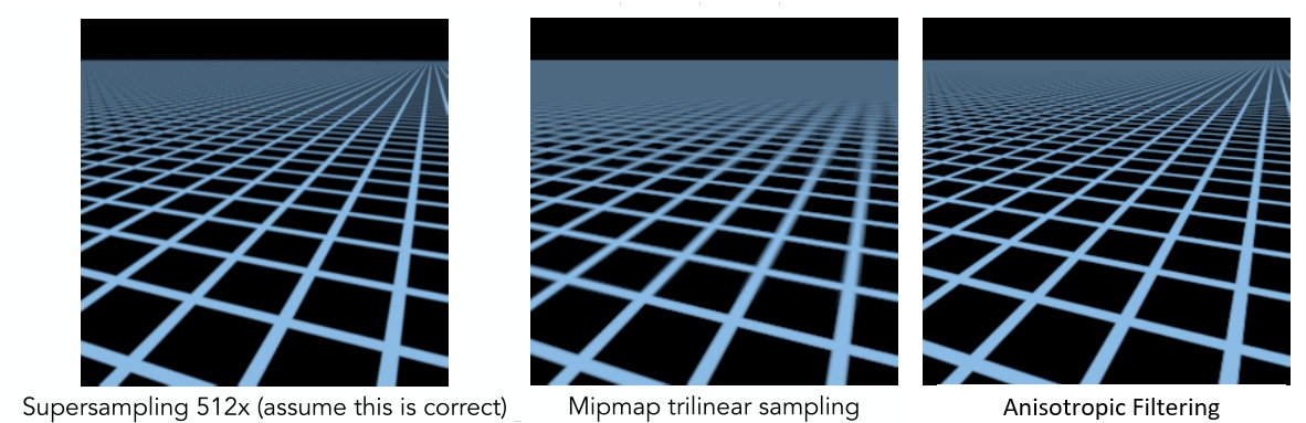
图形学中的纹理映射:高级技巧与优化方法,提升性能的5大策略
# 摘要
本文系统地探讨了纹理映射的基础理论、高级技术和优化方法,以及在提升性能和应用前景方面的策略。纹理映射作为图形渲染中的核心概念,对于增强虚拟场景的真实感和复杂度至关重要。文章首先介绍了纹理映射的基本定义及其重要性,接着详述了不同类型的纹理映射及应用场景。随后,本文深入探讨了高级纹理映射技术,包括纹理压缩、缓存与内存管理和硬件加速,旨在减少资源消耗并提升
【Typora插件应用宝典】:提升写作效率与体验的15个必备插件

# 摘要
本论文详尽探讨了Typora这款Markdown编辑器的界面设计、编辑基础以及通过插件提升写作效率和阅读体验的方法。文章首先介绍了Typora的基本界面与编辑功能,随后深入分析了多种插件如何辅助文档结构整理、代码编写、写作增强、文献管理、多媒体内容嵌入及个性化定制等方面。此外,文章还讨论了插件管理、故障排除以及如何保证使用插件时
RML2016.10a字典文件深度解读:数据结构与案例应用全攻略
# 摘要
本文全面介绍了RML2016.10a字典文件的结构、操作以及应用实践。首先概述了字典文件的基本概念和组成,接着深入解析了其数据结构,包括头部信息、数据条目以及关键字与值的关系,并探讨了数据操作技术。文章第三章重点分析了字典文件在数据存储、检索和分析中的应用,并提供了实践中的交互实例。第四章通过案例分析,展示了字典文件在优化、错误处理、安全分析等方面的应用及技巧。最后,第五章探讨了字典文件的高
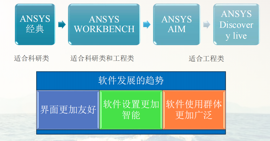
【Ansoft软件精通秘籍】:一步到位掌握电磁仿真精髓
# 摘要
本文详细介绍了Ansoft软件的功能及其在电磁仿真领域的应用。首先概述了Ansoft软件的基本使用和安装配置,随后深入讲解了基础电磁仿真理论,包括电磁场原理、仿真模型建立、仿真参数设置和网格划分的技巧。在实际操作实践章节中,作者通过多个实例讲述了如何使用Ansoft HFSS、Maxwell和Q3D Extractor等工具进行天线、电路板、电机及变压器等的电磁仿真。进而探讨了Ansoft的高级技巧
负载均衡性能革新:天融信背后的6个优化秘密
# 摘要
负载均衡技术是保障大规模网络服务高可用性和扩展性的关键技术之一。本文首先介绍了负载均衡的基本原理及其在现代网络架构中的重要性。继而深入探讨了天融信的负载均衡技术,重点分析了负载均衡算法的选择标准、效率与公平性的平衡以及动态资源分配机制。本文进一步阐述了高可用性设计原理,包括故障转移机制、多层备份策略以及状态同步与一致性维护。在优化实践方面,本文讨论了硬件加速、性能调优、软件架构优化以及基于AI的自适应优化算法。通过案例
【MAX 10 FPGA模数转换器时序控制艺术】:精确时序配置的黄金法则
# 摘要
本文主要探讨了FPGA模数转换器时序控制的基础知识、理论、实践技巧以及未来发展趋势。首先,从时序基础出发,强调了时序控制在保证FPGA性能中的重要性,并介绍了时序分析的基本方法。接着,在实践技巧方面,探讨了时序仿真、验证、高级约束应用和动态时序调整。文章还结合MAX 10 FPGA的案例,详细阐述了模数转换器的
资源上传下载、课程学习等过程中有任何疑问或建议,欢迎提出宝贵意见哦~我们会及时处理!
点击此处反馈


专栏目录
最低0.47元/天 解锁专栏
买1年送3月
百万级
高质量VIP文章无限畅学
千万级
优质资源任意下载
C知道
免费提问 ( 生成式Al产品 )