
Eric Galin et al. / A Review of Digital Terrain Modeling
The method can be generalized to other faulting geometries such
as curves or circles, and scales to any size and can be extended
to generate fractal planets [FFC82b] when applied to a sphere.
[KSU07] proposed a variation of the faulting algorithm to control
the shape of procedurally generated terrain by prescribing control
parameters such as the height and extent of the base region at a
given location.
3.1.3. Noise
Noise functions [Per85,Per89,Wor96, LLDD09] have been widely
studied and used for a variety of natural phenomena, including ter-
rain modeling. A complete description of noise functions is beyond
the scope of this paper, we refer the reader to [LSC
∗
10] for an
overview of procedural noise functions.
Noise functions have been proposed as basis functions for rep-
resenting infinite terrains, i.e. defined over R
2
, as a set of scaled
and warped noise functions [MKM89, EMP
∗
98]. By adding sev-
eral noises at different scales and amplitudes, it is possible to build
a function that locally resembles a real terrain. Fractional Brownian
motion, also sometimes referred to as turbulence and denoted as t,
can be implemented as a combination of multiple steps of noise
each with a different frequency and amplitude. In the context of
procedural generation, the variation in frequency from a step to the
next is called lacunarity, whereas the variation in amplitude from a
step to the next is called gain or persistence.
Let n denote a smooth noise function that maps from R
2
to
[−1,1] interval; without loss of generality we consider that this fun-
damental function has a primary frequency of 1; which means that
it interpolates values or gradients defined at every integer position.
The turbulence function t is defined by summing the contributions
of noises with varying frequencies and amplitudes:
t(p) =
i=o−1
∑
i=0
a
i
n(ϕ
i
p)
where a
i
refer to the different amplitudes, ϕ
i
to the different fre-
quencies. The number of terms o is often referred as the number of
octaves, even if the frequencies are not multiples of 2. In general,
the amplitudes and frequencies are defined as a geometric series:
a
i
= a
0
p
i
and ϕ
i
= ϕ
0
l
i
where a
0
and ϕ
0
are the base amplitude
and frequency, l ∈ [0,1] is the lacunarity, and p ∈ [0, 1] the per-
sistence. The persistence defines how the amplitude decreases in
the successive octaves. Values p ≈ 1 produce very jagged terrains,
whereas values p ≈ 0 drastically limit the impact of the successive
frequencies.
Exponential noise was proposed in [Par15] to better reproduce
the slope distribution observed in real terrains. The exponential
slope distribution spectrum is obtained by analyzing real terrain
data, and used to constrain the generation process using gradi-
ent noise whose gradient samples match the multi-fractal spec-
trum [vLJ95, Par14,Par15].
The smoothness of the noise function n prevents the creation of
crests and ridge lines that can be found in mountainous terrains
(Figure 7 left). Ridge noise was therefore introduced with a view
to generating sharp features such as crests or ridges, and simply
defined as r(p) = 1 − |n(p)|. Although the absolute value was al-
ready present in the definition of the turbulence function in [Per85],
the idea of turning it upside-down to produce crests on the top of
mountain ranges was introduced in [EMP
∗
98].
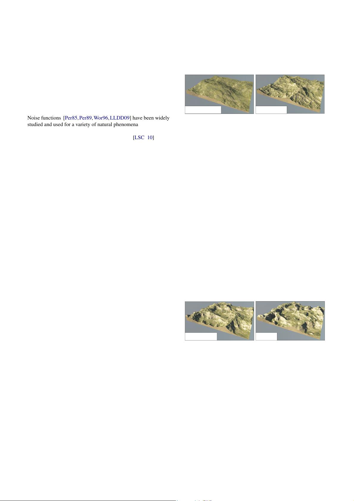
Ridge noise
Simplex noise
Figure 7: A sum of simplex noise n (left) and ridge noise r (right)
with 8 octaves: ridge noise generates crest lines suitable for young
mountains, whereas simplex noise is more suitable to modeling
hills.
The fractal property of these noise functions is uniform, i.e. they
generate mono-fractals, which does not conform to real landscapes.
Multi-fractal terrains can be obtained by modifying the sum of oc-
taves so that the amplitude of higher frequencies a
k+1
should be
weighted by a function α according to value of the previously com-
puted octaves [EMP
∗
98]. This can be obtained by using the fol-
lowing recurrence relation:
t
k+1
(p) = α(t
k
(p))a
k+1
n(ϕ
i
p) +t
k
(p) t
0
(p) = a
0
n(ϕ
0
p)
Lower elevations t
k
(p), computed at step k, scale down higher fre-
quencies in order to smooth valleys, whereas higher values will
boost high frequencies to enhance the mountains peaks with small
details. Multi-fractal generate terrains that are not uniform featur-
ing smooth areas in plains and ridged landforms in mountains (Fig-
ure 8 left).
Summing the same scaled noise function n can lead to grid ar-
tifacts that can be avoided by applying warping functions made
of rotations and translations. This concept is easily formalized
by the means of an affine transformation applied to p, i.e. using
n(R
i
p + v
i
) where R
i
is a 2 × 2 random rotation matrix and v
i
is
the translation vector.
Warped
Multi fractal
Figure 8: A multi-fractal sum of 8 octaves of ridged noises (left)
and its warped version (right).
Warping Generally, warping can be used to deform the domain
and break the monotonicity and regularity of noise. Formally, a
continuous warping function may defined as: ω : R
2
→ R
2
; and
warped terrains are computed by evaluating n ◦ ω(p) instead of
n(p). The warping function ω may be defined as a sum of scaled
displacement functions created from noise. Low frequency vector
offsets are commonly used for this purpose (Figure 8 right). Lim-
ited erosion effects can be approximated [dCB09] by using warp-
ing functions based on scaled noise, oriented in the direction of the
c
2019 The Author(s)
Computer Graphics Forum
c
2019 The Eurographics Association and John Wiley & Sons Ltd.
557
剩余24页未读,继续阅读

tomren
- 粉丝: 13
- 资源: 18
 我的内容管理
展开
我的内容管理
展开


最新资源
- 多模态联合稀疏表示在视频目标跟踪中的应用
- Kubernetes资源管控与Gardener开源软件实践解析
- MPI集群监控与负载平衡策略
- 自动化PHP安全漏洞检测:静态代码分析与数据流方法
- 青苔数据CEO程永:技术生态与阿里云开放创新
- 制造业转型: HyperX引领企业上云策略
- 赵维五分享:航空工业电子采购上云实战与运维策略
- 单片机控制的LED点阵显示屏设计及其实现
- 驻云科技李俊涛:AI驱动的云上服务新趋势与挑战
- 6LoWPAN物联网边界路由器:设计与实现
- 猩便利工程师仲小玉:Terraform云资源管理最佳实践与团队协作
- 类差分度改进的互信息特征选择提升文本分类性能
- VERITAS与阿里云合作的混合云转型与数据保护方案
- 云制造中的生产线仿真模型设计与虚拟化研究
- 汪洋在PostgresChina2018分享:高可用 PostgreSQL 工具与架构设计
- 2018 PostgresChina大会:阿里云时空引擎Ganos在PostgreSQL中的创新应用与多模型存储
资源上传下载、课程学习等过程中有任何疑问或建议,欢迎提出宝贵意见哦~我们会及时处理!
点击此处反馈


