时间序列分解:揭开时间序列数据的秘密结构
发布时间: 2024-08-21 23:05:36 阅读量: 44 订阅数: 37 

淡水:21世纪的分子微生物生态学1

# 1. 时间序列分解概述
时间序列分解是一种将时间序列数据分解为多个组成部分的技术,这些组成部分代表了数据中不同的模式和趋势。通过分解,我们可以更深入地了解数据结构,识别潜在的模式和异常值,并为预测和异常检测提供基础。
时间序列分解的目的是将原始数据分解为以下几个组成部分:
- **趋势:**代表数据中的长期趋势或总体方向。
- **季节性:**代表数据中周期性的模式,例如每周、每月或每年重复的模式。
- **残差:**代表数据中无法用趋势或季节性解释的随机波动。
# 2. 时间序列分解理论
### 2.1 时间序列的组成部分
时间序列可以分解为三个基本组成部分:
- **趋势(Trend):**时间序列中长期变化的总体方向,反映了数据的总体增长或下降趋势。
- **季节性(Seasonality):**时间序列中周期性的波动,与一年中的特定时间或事件相关,如季节、节假日或营业时间。
- **残差(Residual):**时间序列中无法用趋势或季节性解释的随机波动,通常表示不可预测的事件或噪声。
### 2.2 分解方法:加性分解和乘性分解
时间序列分解有两种主要方法:加性分解和乘性分解。
- **加性分解:**假设时间序列的组成部分是相加的,即:
```
Y = T + S + R
```
其中:
- Y:原始时间序列
- T:趋势
- S:季节性
- R:残差
- **乘性分解:**假设时间序列的组成部分是相乘的,即:
```
Y = T * S * R
```
选择加性分解还是乘性分解取决于时间序列数据的特点。如果趋势和季节性是线性的,则使用加性分解;如果趋势和季节性是非线性的,则使用乘性分解。
### 2.3 常用分解算法:滑动平均、指数平滑
常用的时间序列分解算法包括:
- **滑动平均:**一种简单但有效的分解方法,通过计算时间序列中特定窗口内的平均值来估计趋势。
- **指数平滑:**一种加权平均方法,赋予最近的数据点更大的权重,从而对趋势和季节性做出更快的响应。
**滑动平均算法:**
```python
import numpy as np
def moving_average(series, window_size):
"""
计算时间序列的滑动平均。
参数:
series: 时间序列数据。
window_size: 滑动窗口大小。
返回:
滑动平均后的时间序列。
"""
return np.convolve(series, np.ones(window_size) / window_size, mode='valid')
```
**指数平滑算法:**
```python
import statsmodels.api as sm
def exponential_smoothing(series, alpha):
"""
计算时间序列的指数平滑。
参数:
series: 时间序列数据。
alpha: 平滑因子,0 < alpha < 1。
返回:
指数平滑后的时间序列。
"""
return sm.tsa.statespace.ExponentialSmoothing(series, trend='add', seasonal=None).fit(smoothing_level=alpha).fittedvalues
```
**代码逻辑分析:**
- **滑动平均:**`np.convolve()`函数执行卷积操作,将时间序列与一个均匀分布的窗口进行卷积,从而计算滑动平均。
- **指数平滑:**`ExponentialSmoothing`类使用卡尔曼滤波器实现指数平滑,`smoothing_level`参数指定平滑因子,控制对当前数据的权重。
# 3. 时间序列分解实践
### 3.1 使用Python进行时间序列分解
#### 导入必要的库
```python
import numpy as np
import pandas as pd
from statsmodels.tsa.statespace. sarimax import SARIMAX
from statsmodels.tsa.seasonal import seasonal_decompose
```
#### 加载时间序列数据
```python
# 加载CSV文件中的时间序列数据
data = pd.read_csv('time_series_data.csv', index_col='Date', parse_dates=True)
# 指定时间序列列
ts = data['value']
```
#### 滑动平均分解
```python
# 滑动平均分解
decomposition = seasonal_decompose(ts, model='additive', period=7)
# 获取分解后的成分
trend = decomposition.trend
seasonal = decomposition.seasonal
residual = decomposition.resid
```
#### 指数平滑分解
```python
# 指数平滑分解
decomposition = seasonal_decompose(ts, model='additive', method='ets')
# 获取分解后的成分
trend = decomposition.trend
seasonal = decomposition.seasonal
residual = decomposition.resid
```
### 3.2 分解结果的分析和解释
#### 趋势成分
趋势成分代表时间序列的长期趋势,通常是上升或下降的平滑曲线。它可以揭示时间序列的整体变化模式。
#### 季节性成分
季节性成分表示时间序列中重复出现的周期性模式,通常与一年中的时间或其他周期性事件相关。它可以帮助识别时间序列中的季节性波动。
#### 残差成分
残差成分是时间序列中无法通过趋势和季节性成分解释的部分。它通常包含随机波动和异常值,可以提供时间序列中未被建模模式捕获的额外信息。
#### 分解结果的可视化
```python
# 绘制分解结果
decomposition.plot()
plt.show()
```
可视化分解结果可以直观地显示时间序列的组成部分,并有助于识别趋势、季节性和残差模式。
# 4. 时间序列分解在预测中的应用
### 4.1 分解预测法
时间序列分解预测法是一种基于时间序列分解结果进行预测的方法。其基本思想是将时间序列分解为趋势、季节性、残差等组成部分,然后分别对这些组成部分进行预测,最后将预测结果相加得到最终的预测值。
**步骤:**
1. 将时间序列分解为趋势、季节性、残差等组成部分。
2. 对每个组成部分进行预测。
3. 将预测结果相加得到最终的预测值。
**优点:**
* 分解预测法可以利用时间序列的不同组成部分的特性进行预测,提高预测精度。
* 分解预测法可以识别时间序列中不同的模式,为预测提供更多信息。
**缺点:**
* 分解预测法对分解算法的选择敏感,不同的分解算法可能会导致不同的预测结果。
* 分解预测法对预测期间的长度敏感,预测期间越长,预测精度越低。
### 4.2 趋势预测和季节性预测
**趋势预测**
趋势预测是指对时间序列中趋势部分的预测。趋势预测的方法有很多,常用的方法包括:
* 移动平均法
* 指数平滑法
* ARIMA模型
**季节性预测**
季节性预测是指对时间序列中季节性部分的预测。季节性预测的方法有很多,常用的方法包括:
* 季节性指数平滑法
* 傅里叶变换
* ARIMA模型
**示例:**
假设我们有一个销售时间序列,该时间序列具有明显的趋势和季节性。我们可以使用分解预测法对该时间序列进行预测。
**步骤:**
1. 使用滑动平均法分解时间序列为趋势、季节性、残差三部分。
2. 使用指数平滑法对趋势部分进行预测。
3. 使用季节性指数平滑法对季节性部分进行预测。
4. 将趋势预测值和季节性预测值相加得到最终的预测值。
**代码块:**
```python
import pandas as pd
import statsmodels.api as sm
import matplotlib.pyplot as plt
# 加载数据
data = pd.read_csv('sales.csv')
# 分解时间序列
decomposition = sm.tsa.seasonal_decompose(data['sales'], model='additive')
# 趋势预测
trend_forecast = sm.tsa.statespace.SARIMAX(decomposition.trend, order=(1, 1, 0), seasonal_order=(1, 1, 0, 12)).fit().forecast(steps=12)
# 季节性预测
seasonal_forecast = sm.tsa.statespace.SARIMAX(decomposition.seasonal, order=(0, 1, 1), seasonal_order=(1, 1, 0, 12)).fit().forecast(steps=12)
# 最终预测
forecast = trend_forecast + seasonal_forecast
# 绘制预测结果
plt.plot(data['sales'], label='实际值')
plt.plot(forecast, label='预测值')
plt.legend()
plt.show()
```
**逻辑分析:**
* `sm.tsa.seasonal_decompose()`函数使用滑动平均法对时间序列进行分解,得到趋势、季节性、残差三部分。
* `sm.tsa.statespace.SARIMAX()`函数使用指数平滑法对趋势部分进行预测。
* `sm.tsa.statespace.SARIMAX()`函数使用季节性指数平滑法对季节性部分进行预测。
* `forecast = trend_forecast + seasonal_forecast`将趋势预测值和季节性预测值相加得到最终的预测值。
**参数说明:**
* `order`参数指定ARIMA模型的阶数。
* `seasonal_order`参数指定季节性ARIMA模型的阶数。
* `steps`参数指定预测的步长。
# 5. 时间序列分解在异常检测中的应用**
**5.1 异常检测原理**
异常检测是一种识别与正常模式显著不同的数据点的技术。在时间序列分析中,异常可以表示为偏离预期模式或趋势的观察值。
**5.2 基于分解的异常检测算法**
基于分解的异常检测算法利用时间序列分解将数据分解为不同的组成部分,然后分析这些组成部分以识别异常。以下是一些常用的基于分解的异常检测算法:
**5.2.1 残差分析**
残差分析涉及计算观测值与分解模型预测值之间的差值。异常值通常表现为残差值明显高于或低于预期范围。
**5.2.2 趋势分析**
趋势分析着眼于时间序列的趋势分量。异常值可能表现为趋势的突然变化或中断。
**5.2.3 季节性分析**
季节性分析关注时间序列的季节性分量。异常值可能表现为季节性模式的异常或缺失。
**5.2.4 异常检测流程**
基于分解的异常检测流程通常包括以下步骤:
1. **分解时间序列:**使用滑动平均、指数平滑或其他分解算法将时间序列分解为趋势、季节性和残差分量。
2. **设置阈值:**确定异常值的阈值,例如残差值的标准差或趋势变化的百分比。
3. **识别异常:**将超出阈值的观察值标记为异常值。
4. **分析异常:**调查异常值以确定其潜在原因,例如数据错误、异常事件或模式变化。
**代码示例:**
```python
import numpy as np
import pandas as pd
from statsmodels.tsa.seasonal import seasonal_decompose
# 加载时间序列数据
data = pd.read_csv('time_series_data.csv')
# 分解时间序列
decomposition = seasonal_decompose(data['value'], model='additive')
# 计算残差
residuals = data['value'] - decomposition.resid
# 设置阈值
threshold = 2 * np.std(residuals)
# 识别异常值
anomalies = residuals[abs(residuals) > threshold]
# 打印异常值
print(anomalies)
```
**逻辑分析:**
此代码示例演示了基于分解的异常检测流程:
* 时间序列数据被分解为趋势、季节性和残差分量。
* 残差值被计算出来,并用标准差设置阈值。
* 超出阈值的残差值被标记为异常值。
* 最后,异常值被打印出来,以便进一步分析。
# 6. 时间序列分解在金融领域的应用
### 6.1 金融时间序列的特点
金融时间序列数据具有以下特点:
- **高波动性:**金融资产价格受多种因素影响,波动较大。
- **非平稳性:**金融时间序列的均值和方差会随时间变化。
- **季节性:**金融市场存在明显的季节性规律,如月度、季度和年度周期。
- **周期性:**金融时间序列往往存在周期性波动,如经济周期和市场周期。
### 6.2 分解在金融风险管理和投资决策中的作用
时间序列分解在金融领域有着广泛的应用,主要体现在以下方面:
**金融风险管理:**
- **风险评估:**通过分解金融时间序列,可以识别和量化风险因素,如市场波动、利率变化和经济衰退。
- **压力测试:**基于分解结果,可以模拟极端市场条件下的金融资产表现,评估金融机构的抗风险能力。
**投资决策:**
- **趋势识别:**分解可以帮助识别金融资产的长期趋势,为投资决策提供依据。
- **季节性调整:**通过分解可以去除金融时间序列中的季节性影响,更准确地评估资产的真实表现。
- **周期性预测:**分解可以帮助预测金融资产的周期性波动,把握市场时机。
### 应用示例
**股票价格预测:**
股票价格是一个典型的高波动性、非平稳时间序列。通过分解股票价格时间序列,可以识别其趋势、季节性和周期性成分。基于这些成分,可以建立预测模型,预测股票价格的未来走势。
**债券收益率预测:**
债券收益率时间序列具有较强的季节性和周期性。通过分解债券收益率时间序列,可以识别其长期趋势和短期波动。基于这些成分,可以建立预测模型,预测债券收益率的未来走势,为投资决策提供指导。

 百万级
高质量VIP文章无限畅学
百万级
高质量VIP文章无限畅学
 千万级
优质资源任意下载
千万级
优质资源任意下载
 C知道
免费提问 ( 生成式Al产品 )
C知道
免费提问 ( 生成式Al产品 )
0
0
相关推荐

专栏简介
时间序列分解方法专栏深入探讨了时间序列数据的分解技术,揭示了其作为预测模型秘密武器的强大力量。通过一系列标题,专栏全面介绍了时间序列分解的各个方面,从入门到精通预测模型构建。它揭示了数据背后的结构,包括季节性变化、残差波动和长期趋势。专栏强调了时间序列分解在提升预测准确性、识别异常值、数据可视化和机器学习特征工程中的关键作用。它还提供了从理论基础到实际应用的完整指南,涵盖了从业者的必备技能和最佳实践。通过深入了解时间序列分解,数据科学家和分析师可以掌握应对数据复杂性的有效策略,并提升其数据分析能力。
专栏目录
最低0.47元/天 解锁专栏
买1年送3月
百万级
高质量VIP文章无限畅学
千万级
优质资源任意下载
C知道
免费提问 ( 生成式Al产品 )
最新推荐
C# WinForm程序打包进阶秘籍:掌握依赖项与配置管理
# 摘要
本文系统地探讨了WinForm应用程序的打包过程,详细分析了依赖项管理和配置管理的关键技术。首先,依赖项的识别、分类、打包策略及其自动化管理方法被逐一介绍,强调了静态与动态链接的选择及其在解决版本冲突中的重要性。其次,文章深入讨论了应用程序配置的基础和高级技巧,如配置信息的加密和动态加载更新。接着,打包工具的选择、自动化流程优化以及问题诊断与解决策略被详细
参数设置与优化秘籍:西门子G120变频器的高级应用技巧揭秘

# 摘要
西门子G120变频器是工业自动化领域的关键设备,其参数配置对于确保变频器及电机系统性能至关重要。本文旨在为读者提供一个全面的西门子G120变频器参数设置指南,涵盖了从基础参数概览到高级参数调整技巧。本文首先介绍了参数的基础知识,包括各类参数的功能和类
STM8L151 GPIO应用详解:信号控制原理图解读

# 摘要
本文详细探讨了STM8L151微控制器的通用输入输出端口(GPIO)的功能、配置和应用。首先,概述了GPIO的基本概念及其工作模式,然后深入分析了其电气特性、信号控制原理以及编程方法。通过对GPIO在不同应用场景下的实践分析,如按键控制、LED指示、中断信号处理等,文章揭示了GPIO编程的基础和高级应
【NI_Vision进阶课程】:掌握高级图像处理技术的秘诀
# 摘要
本文详细回顾了NI_Vision的基本知识,并深入探讨图像处理的理论基础、颜色理论及算法原理。通过分析图像采集、显示、分析、处理、识别和机器视觉应用等方面的实际编程实践,本文展示了NI_Vision在这些领域的应用。此外,文章还探讨了NI_Vision在立体视觉、机器学习集成以及远程监控图像分析中的高级功能。最后,通过智能监控系统、工业自动化视觉检测和医疗图像处理应用等项目案例,
【Cortex R52与ARM其他处理器比较】:全面对比与选型指南
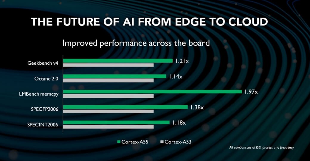
# 摘要
本文详细介绍了Cortex R52处理器的架构特点、应用案例分析以及选型考量,并提出了针对Cortex R52的优化策略。首先,文章概述了Cortex R52处理器的基本情
JLINK_V8固件烧录安全手册:预防数据损失和设备损坏
# 摘要
本文对JLINK_V8固件烧录的过程进行了全面概述,包括烧录的基础知识、实践操作、安全防护措施以及高级应用和未来发展趋势。首先,介绍了固件烧录的基本原理和关键技术,并详细说明了JLINK_V8烧录器的硬件组成及其操作软件和固件。随后,本文阐述了JLINK_V8固件烧录的操作步骤,包括烧录前的准备工作和烧录过程中的操作细节,并针对常见问题提供了相应的解决方法。此外,还探讨了数据备份和恢
Jetson Nano性能基准测试:评估AI任务中的表现,数据驱动的硬件选择

# 摘要
Jetson Nano作为一款针对边缘计算设计的嵌入式设备,其性能和能耗特性对于AI应用至关重要。本文首先概述了Jetson Nano的硬件架构,并强调了性能基准测试在评估硬件性能中的重要性。通过分析其处理器、内存配置、能耗效率和散热解决方案,本研究旨在提供详尽的硬件性能基准测试方法,并对Jetson Nano在不同AI任务中的表现进行系统评估。最
MyBatis-Plus QueryWrapper多表关联查询大师课:提升复杂查询的效率

# 摘要
本文围绕MyBatis-Plus框架的深入应用,从安装配置、QueryWrapper使用、多表关联查询实践、案例分析与性能优化,以及进阶特性探索等几个方面进行详细论述。首先介绍了MyBatis-Plus的基本概念和安装配置方法。随
【SAP BW4HANA集成篇】:与S_4HANA和云服务的无缝集成

# 摘要
随着企业数字化转型的不断深入,SAP BW4HANA作为新一代的数据仓库解决方案,在集成S/4HANA和云服务方面展现了显著的优势。本文详细阐述了SAP BW4HANA集成的背景、优势、关键概念以及业务需求,探讨了与S/4HANA集成的策略,包括集成架构设计、数据模型适配转换、数据同步技术与性能调优。同时,本文也深入分析了SAP BW4HANA与云服务集成的实
资源上传下载、课程学习等过程中有任何疑问或建议,欢迎提出宝贵意见哦~我们会及时处理!
点击此处反馈


专栏目录
最低0.47元/天 解锁专栏
买1年送3月
百万级
高质量VIP文章无限畅学
千万级
优质资源任意下载
C知道
免费提问 ( 生成式Al产品 )