Best Practices for Solving Linear Equations with MATLAB Matrices: Improving Efficiency by Choosing the Right Method, 3 Common Approaches
发布时间: 2024-09-15 01:37:16 阅读量: 38 订阅数: 39 

Two Scoops of Django 1.11: Best Practices for the Django Web Framework.pdf
# Best Practices for Solving Linear Equations with MATLAB: Choosing the Right Method for Efficiency, 3 Common Approaches
## 1. Fundamentals of Solving Linear Equations in MATLAB
Linear equation systems are a common problem in mathematics that involve finding a set of unknown variables satisfying a series of linear equations. MATLAB offers a suite of powerful tools to solve linear equation systems, including direct and iterative methods.
In this chapter, we will cover the basic knowledge of solving linear equation systems in MATLAB. We will discuss the mathematical model of linear equation systems and introduce the two main methods of solving linear equation systems in MATLAB: direct methods and iterative methods.
## 2. Theoretical Foundations of Solving Linear Equation Systems in MATLAB
### 2.1 Mathematical Model of Linear Equation Systems
Linear equation systems are a set of equations in the following form:
```
a11x1 + a12x2 + ... + a1nxn = b1
a21x1 + a22x2 + ... + a2nxn = b2
am1x1 + am2x2 + ... + amnxn = bm
```
Where `aij` are the elements of the coefficient matrix, `x1`, `x2`, ..., `xn` are the unknowns, and `b1`, `b2`, ..., `bm` are the elements of the constant vector.
### 2.2 Matrix Inversion Method
The matrix inversion method is a direct method for solving linear equation systems. It obtains the unknowns by inverting the coefficient matrix.
**Steps:**
1. Write the linear equation system in matrix form: `Ax = b`, where `A` is the coefficient matrix, `x` is the unknown vector, and `b` is the constant vector.
2. Find the inverse of the coefficient matrix `A`, `A^-1`.
3. Solve for the unknown vector: `x = A^-1b`.
**Code Example:**
```matlab
% Coefficient matrix
A = [2 1; 3 4];
% Constant vector
b = [5; 11];
% Calculate the inverse of the coefficient matrix
A_inv = inv(A);
% Solve for the unknown vector
x = A_inv * b;
% Display the result
disp(x);
```
**Logical Analysis:**
* The `inv(A)` function is used to calculate the inverse matrix of `A`.
* `x = A_inv * b` computes the unknown vector `x`.
### 2.3 Cramer's Rule
Cramer's rule is another direct method for solving linear equation systems. It obtains the unknowns by calculating the Cramer determinant for each unknown.
**Cramer Determinant:**
For an unknown `xi`, its Cramer determinant is:
```
C_i = det(A_i) / det(A)
```
Where `A_i` is the matrix with the `i`th column replaced by the constant vector `b`, and `det(A)` is the determinant of the coefficient matrix `A`.
**Steps:**
1. Calculate the determinant of the coefficient matrix `A`.
2. For each unknown `xi`, calculate its Cramer determinant `C_i`.
3. Solve for the unknown: `xi = C_i / det(A)`.
**Code Example:**
```matlab
% Coefficient matrix
A = [2 1; 3 4];
% Constant vector
b = [5; 11];
% Calculate the determinant of the coefficient matrix
det_A = det(A);
% Calculate the Cramer determinant for each unknown
C1 = det([b, 1; 3, 4]);
C2 = det([2, b; 3, 11]);
% Solve for the unknowns
x1 = C1 / det_A;
x2 = C2 / det_A;
% Display the result
disp([x1, x2]);
```
**Logical Analysis:**
* The `det(A)` function calculates the determinant of the matrix `A`.
* `det([b, 1; 3, 4])` calculates the Cramer determinant for the unknown `x1`.
* `det([2, b; 3, 11])` calculates the Cramer determinant for the unknown `x2`.
## 3.1 Direct Solution Methods
Direct solution methods involve a series of operations on the coefficient matrix of the linear equation system to transform it into an upper triangular or diagonal matrix, and then solve the equation system through back substitution. Direct solution methods mainly include Gauss elimination and LU decomposition.
#### 3.1.1 Gauss Elimination Method
The Gauss elimination method is a classic direct solution method. Its basic idea is to transform the coefficient matrix into an upper triangular matrix through row transformations, and then solve the equation system through back substitution. The specific steps of the Gauss elimination method are as follows:
1. **Elimination:** Starting with the first equation, perform elimination operations on each equation in turn, i.e., multiply the coefficients of that equation by the corresponding coefficients of other equations and add them to obtain a new equation system. In this new system, the first equation contains only one unknown, the second equation contains only two unknowns, and so on.
2. **Back substitution:** Starting with the last equation, perform back substitution operations on each equation in turn, i.e., use the values of the known unknowns to solve for the values of other unknowns.
Gauss elimination method code example:
```matlab
% Given coefficient matrix A and right-hand vector b
A = [2 1 1; 4 3 2; 8 7 4];
b = [1; 2; 3];
% Perform Gauss elimination
for i = 1:size(A, 1)
```

 百万级
高质量VIP文章无限畅学
百万级
高质量VIP文章无限畅学
 千万级
优质资源任意下载
千万级
优质资源任意下载
 C知道
免费提问 ( 生成式Al产品 )
C知道
免费提问 ( 生成式Al产品 )
0
0
相关推荐

专栏目录
最低0.47元/天 解锁专栏
买1年送3月
百万级
高质量VIP文章无限畅学
千万级
优质资源任意下载
C知道
免费提问 ( 生成式Al产品 )
最新推荐
【GP系统集成实战】:将GP Systems Scripting Language无缝融入现有系统

# 摘要
GP系统脚本语言作为一种集成和自动化工具,在现代企业信息系统中扮演着越来越重要的角色。本文首先概述了GP系统脚本语言的核心概念及其集成的基础理论,包括语法结构、执行环境和系统集成的设计原则。随后,文章深入探讨了GP系统集成的实战技巧,涵盖数据库集成、网络功能、企业级应用实践等方面。此外,本文还分析了GP系统集成在高
【Twig模板性能革命】:5大技巧让你的Web飞速如风

# 摘要
Twig作为一款流行的模板引擎,在现代Web开发中扮演着重要角色,它通过高效的模板语法和高级特性简化了模板的设计和维护工作。本文从Twig的基本语法开始,逐步深入到性能优化和实际应用技巧,探讨了模板继承、宏的使用、自定义扩展、
【正确方法揭秘】:爱普生R230废墨清零,避免错误操作,提升打印质量
# 摘要
废墨清零是确保打印机长期稳定运行的关键维护步骤,对于保障打印质量和设备性能具有重要的基础作用。本文系统介绍了废墨清零的基础知识、操作原理、实践操作以及其对打印质量的影响。通过对废墨产生、积累机制的理解,本文阐述了废墨清零的标准操作步骤和准备工作,同时探讨了实践中可能遇到的问题及其解决方法。文章还分析了废墨清零操作如何正面影响打印质量,并提出了避免错误操作的建议。最后,本文探讨了其他提升打印质量的方法和技巧,包括硬件选择、日常维护
【降噪耳机功率管理】:优化电池使用,延长续航的权威策略

# 摘要
本文全面探讨了降噪耳机的功率管理问题,从理论基础到实践应用,再到未来发展趋势进行了系统性的分析。首先介绍了降噪耳机功率消耗的现状,并探讨了电池技术与功耗管理系统设计原则。随后,文章深入到硬件节能技术、软件算法以及用户交互等方面的实际功率管
避免K-means陷阱:解决初始化敏感性问题的实用技巧
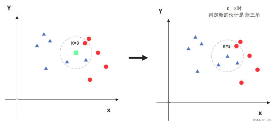
# 摘要
K-means聚类算法作为一种广泛使用的无监督学习方法,在数据分析和模式识别领域中发挥着重要作用。然而,其初始化过程中的敏感性问题可能导致聚类结果不稳定和质量不一。本文首先介绍了K-means算法及其初始化问题,随后探讨了初始化敏感性的影响及传统方法的不足。接着,文章分析了聚类性能评估标准,并提出了优化策略,包括改进初始化方法和提升聚类结果的稳定性。在此基础上,本文还展示了改进型K-means
STM32 CAN扩展应用宝典:与其他通信协议集成的高级技巧

# 摘要
本论文重点研究了STM32微控制器在不同通信协议集成中的应用,特别是在CAN通信领域的实践。首先介绍了STM32与CAN通信的基础知识,然后探讨了与其他通信协议如RS232/RS485、以太网以及工业现场总线的集成理论和实践方法。详细阐述了硬件和软件的准备、数据传输、错误处理、安全性增强等关键技术点。本文还提供了在STM32平台上实现高性能网络通信的高
ARCGIS分幅图打印神技:高质量输出与分享的秘密
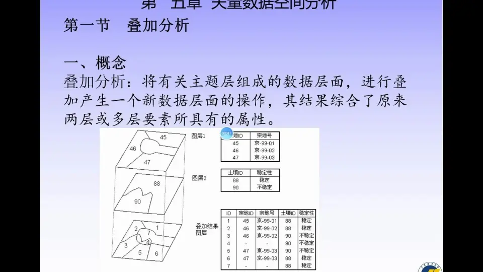
# 摘要
ARCGIS分幅图打印在地图制作和输出领域占据重要地位,本论文首先概述了分幅图打印的基本概念及其在地图输出中的作用和标准规范。随后,深入探讨了分幅图设计的原则,包括用户界面体验与输出质量效率的平衡,以及打印的技术要求,例如分辨率选择和色彩管理。接着,本文提供了分幅图制作和打印的实践技巧,包括数据处理、模板应用、打印设置及输出保存方法。
【install4j更新机制深度剖析】:自动检测与安装更新的高效方案
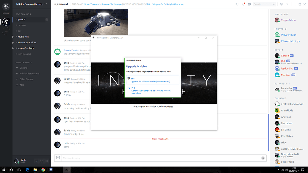
# 摘要
随着软件维护和分发需求的增加,自动更新工具的开发变得日益重要。本文对install4j更新机制进行了全面的分析,介绍了其市场定位和更新流程的必要性。文章深入解析了update检测机制、安装步骤以及更新后应用程序的行为,并从理论基础和实践案例两个维度探讨
【多网络管理】:Quectel-CM模块的策略与技巧

# 摘要
随着物联网技术的发展,多网络管理的重要性日益凸显,尤其是在确保设备在网络间平滑切换、高效传输数据方面。本文首先强调多网络管理的必要性及其应用场景,接着详细介绍Quectel-CM模块的硬件与软件架构。文章深入探讨了基于Quectel-CM模块的网络管理策略,包括网络环境配置、状态监控、故
【ETL与数据仓库】:Talend在ETL过程中的应用与数据仓库深层关系
# 摘要
随着信息技术的不断发展,ETL(提取、转换、加载)与数据仓库已成为企业数据处理和决策支持的重要技术。本文首先概述了ETL与数据仓库的基础理论,明确了ETL过程的定义、作用以及数据抽取、转换和加载的原理,并介绍了数据仓库的架构及其数据模型。随后,本文深入探讨了Talen
资源上传下载、课程学习等过程中有任何疑问或建议,欢迎提出宝贵意见哦~我们会及时处理!
点击此处反馈


专栏目录
最低0.47元/天 解锁专栏
买1年送3月
百万级
高质量VIP文章无限畅学
千万级
优质资源任意下载
C知道
免费提问 ( 生成式Al产品 )