Solving Linear Equations with MATLAB Matrices: 3 Methods, Exploring Different Solution Paths
发布时间: 2024-09-15 01:24:52 阅读量: 31 订阅数: 39 

Matlab Tutorial - 50 - Solving Systems of Linear Equations.zip
# Solving Linear Equations with MATLAB: 3 Methods, Exploring Diverse Solution Paths
## 1. Overview of Linear Equation Systems
Linear equation systems are common mathematical problems that have broad applications in science, engineering, and finance. There are various methods to solve linear equation systems, each with its own advantages and disadvantages.
In MATLAB, the main approaches to solving linear equation systems are direct methods, iterative methods, and Singular Value Decomposition (SVD). Direct methods simplify the coefficient matrix into an upper triangular or diagonal matrix through a series of elementary transformations, and then solve the equation system by back substitution. Iterative methods repeatedly update the approximate values of the unknowns until certain convergence criteria are met. SVD decomposes the coefficient matrix into the product of three matrices, and then uses the decomposed matrices to solve the equation system.
## 2. Methods for Solving Linear Equations in MATLAB
MATLAB provides various methods for solving linear equation systems, including direct methods, iterative methods, and Singular Value Decomposition (SVD).
### 2.1 Direct Methods
Direct methods simplify the coefficient matrix into an upper triangular or diagonal matrix through a series of elementary row operations, and then solve the equation system by back substitution from top to bottom.
#### 2.1.1 Gauss Elimination Method
Gauss Elimination is a classical direct method. Its basic idea is to transform the coefficient matrix into an upper triangular matrix through row operations, and then solve it by back substitution from top to bottom.
**Code Example:**
```matlab
% Coefficient matrix
A = [2, 1, 1; 4, 3, 2; 8, 7, 4];
% Right-hand side constant vector
b = [4; 10; 22];
% Solving using Gauss Elimination
x = gauss(A, b);
% Displaying the solution vector
disp(x);
```
**Logical Analysis:**
* The `gauss()` function implements Gauss Elimination to solve linear equations.
* The function first performs elementary row operations on the coefficient matrix to simplify it into an upper triangular matrix.
* Then, it back substitutes to solve for the unknowns from top to bottom.
#### 2.1.2 LU Decomposition Method
LU Decomposition is a direct method that decomposes the coefficient matrix into the product of a lower triangular matrix and an upper triangular matrix, then solves each of these triangular matrices' systems.
**Code Example:**
```matlab
% Coefficient matrix
A = [2, 1, 1; 4, 3, 2; 8, 7, 4];
% Right-hand side constant vector
b = [4; 10; 22];
% LU Decomposition
[L, U] = lu(A);
% Solving Ly = b
y = L \ b;
% Solving Ux = y
x = U \ y;
% Displaying the solution vector
disp(x);
```
**Logical Analysis:**
* The `lu()` function decomposes the coefficient matrix into lower triangular matrix `L` and upper triangular matrix `U`.
* It then solves `Ly = b` and `Ux = y` separately to obtain the unknowns' solution vector `x`.
### 2.2 Iterative Methods
Iterative methods update the approximate solutions of unknowns through continuous iterations until certain convergence criteria are met.
#### 2.2.1 Jacobi Iterative Method
Jacobi Iterative Method is an iterative method that breaks the linear equation system into multiple subsystems and then solves each subsystem one by one.
**Code Example:**
```matlab
% Coefficient matrix
A = [2, 1, 1; 4, 3, 2; 8, 7, 4];
% Right-hand side constant vector
b = [4; 10; 22];
% Solving using Jacobi Iterative Method
x = jacobi(A, b, 100, 1e-6);
% Displaying the solution vector
disp(x);
```
**Logical Analysis:**
* The `jacobi()` function implements the Jacobi Iterative Method to solve linear equations.
* The function sets the maximum number of iterations and convergence precision.
* During each iteration, the function updates the approximate solutions of each unknown until the convergence conditions are met.
#### 2.2.2 Gauss-Seidel Iterative Method
Gauss-Seidel Iterative Method is an iterative method that, unlike the Jacobi method, uses the latest approximate solution to update each unknown, rather than the approximation from the previous iteration.
**Code Example:**
```matlab
% Coefficient matrix
A = [2, 1, 1; 4, 3, 2; 8, 7, 4];
% Right-hand side constant vector
b = [4; 10; 22];
% Solving using Gauss-Seidel Iterative Method
x = gaussSeidel(A, b, 100, 1e-6);
% Displaying the solution vector
disp(x);
```
**Logical Analysis:**
* The `gaussSeidel()` function implements the Gauss-Seidel Iterative Method to solve linear equations.
* The function sets the maximum number of iterations and convergence precision.
* During each iteration, the function updates the approximate solutions

 百万级
高质量VIP文章无限畅学
百万级
高质量VIP文章无限畅学
 千万级
优质资源任意下载
千万级
优质资源任意下载
 C知道
免费提问 ( 生成式Al产品 )
C知道
免费提问 ( 生成式Al产品 )
0
0
相关推荐

专栏目录
最低0.47元/天 解锁专栏
买1年送3月
百万级
高质量VIP文章无限畅学
千万级
优质资源任意下载
C知道
免费提问 ( 生成式Al产品 )
最新推荐
【色彩调校艺术】:揭秘富士施乐AWApeosWide 6050色彩精准秘诀!
# 摘要
本文探讨了色彩调校艺术的基础与原理,以及富士施乐AWApeosWide 6050设备的功能概览。通过分析色彩理论基础和色彩校正的实践技巧,本文深入阐述了校色工具的使用方法、校色曲线的应用以及校色过程中问题的解决策略。文章还详细介绍了软硬件交互、色彩精准的高级应用案例,以及针对特定行业的色彩调校解决方案。最后,本文展望了色彩调校技术的未来趋势,包括AI在色彩管理中的应用、新兴色彩技术的发
【TwinCAT 2.0实时编程秘技】:5分钟让你的自动化程序飞起来
.png)
# 摘要
TwinCAT 2.0作为一种实时编程环境,为自动化控制系统提供了强大的编程支持。本文首先介绍了TwinCAT 2.0的基础知识和实时编程架构,详细阐述了其软件组件、实时任务管理及优化和数据交换机制。随后,本文转向实际编程技巧和实践,包括熟悉编程环
【混沌系统探测】:李雅普诺夫指数在杜芬系统中的实际案例研究
# 摘要
混沌理论是研究复杂系统动态行为的基础科学,其中李雅普诺夫指数作为衡量系统混沌特性的关键工具,在理解系统的长期预测性方面发挥着重要作用。本文首先介绍混沌理论和李雅普诺夫指数的基础知识,然后通过杜芬系统这一经典案例,深入探讨李雅普诺夫指数的计算方法及其在混沌分析中的作用。通过实验研究,本文分析了李雅普诺夫指数在具体混沌系统中的应用,并讨论了混沌系统探测的未来方向与挑战,特别是在其他领域的扩展应用以及当前研究的局限性和未来研究方向。
# 关键字
混沌理论;李雅普诺夫指数;杜芬系统;数学模型;混沌特性;实验设计
参考资源链接:[混沌理论探索:李雅普诺夫指数与杜芬系统](https://w
【MATLAB数据预处理必杀技】:C4.5算法成功应用的前提

# 摘要
本文系统地介绍了MATLAB在数据预处理中的应用,涵盖了数据清洗、特征提取选择、数据集划分及交叉验证等多个重要环节。文章首先概述了数据预处理的概念和重要性,随后详细讨论了缺失数据和异常值的处理方法,以及数据标准化与归一化的技术。特征提取和选择部分重点介绍了主成分分析(PCA)、线性判别分析(LDA)以及不同特征选择技术的应用。文章还探讨了如何通过训练集和测试集的划分,以及K折
【宇电温控仪516P物联网技术应用】:深度连接互联网的秘诀
# 摘要
宇电温控仪516P作为一款集成了先进物联网技术的温度控制设备,其应用广泛且性能优异。本文首先对宇电温控仪516P的基本功能进行了简要介绍,并详细探讨了物联网技术的基础知识,包括物联网技术的概念、发展历程、关键组件,以及安全性和相关国际标准。继而,重点阐述了宇电温控仪516P如何通过硬件接口、通信协议以
【MATLAB FBG仿真进阶】:揭秘均匀光栅仿真的核心秘籍
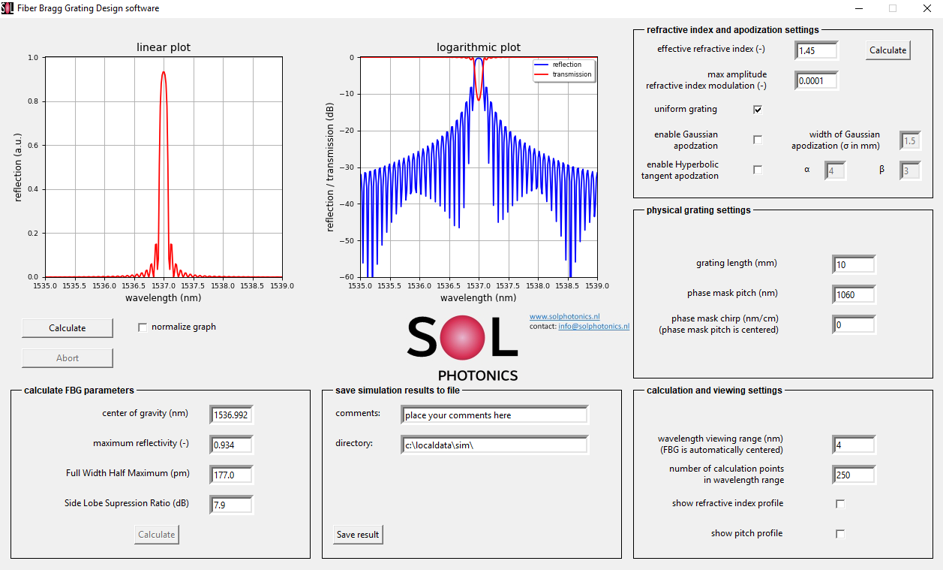
# 摘要
本文全面介绍了基于MATLAB的光纤布喇格光栅(FBG)仿真技术,从基础理论到高级应用进行了深入探讨。首先介绍了FBG的基本原理及其仿真模型的构建方法,包括光栅结构、布拉格波长计算、仿真环境配置和数值分析方法。然后,通过仿真实践分析了FBG的反射和透射特性,以
【ROS2精通秘籍】:2023年最新版,从零基础到专家级全覆盖指南
# 摘要
本文介绍了机器人操作系统ROS2的基础知识、系统架构、开发环境搭建以及高级编程技巧。通过对ROS2的节点通信、参数服务器、服务模型、多线程、异步通信、动作库使用、定时器及延时操作的详细探讨,展示了如何在实践中搭建和管理ROS2环境,并且创建和使用自定义的消息与服务。文章还涉及了ROS2的系统集成、故障排查和性能分析,以
从MATLAB新手到高手:Tab顺序编辑器深度解析与实战演练
# 摘要
本文详细介绍了MATLAB Tab顺序编辑器的使用和功能扩展。首先概述了编辑器的基本概念及其核心功能,包括Tab键控制焦点转移和顺序编辑的逻辑。接着,阐述了界面布局和设置,以及高级特性的实现,例如脚本编写和插件使用。随后,文章探讨了编辑器在数据分析中的应用,重点介绍了数据导入导出、过滤排序、可视化等操作。在算法开发部分,提出了算法设计、编码规范、调试和优化的实战技巧,并通过案例分析展示了算法的实际应用。最后,本文探讨了如何通过创建自定义控件、交互集成和开源社区资源来扩展编辑器功能。
# 关键字
MATLAB;Tab顺序编辑器;数据分析;算法开发;界面布局;功能扩展
参考资源链接:
数据安全黄金法则:封装建库规范中的安全性策略

# 摘要
数据安全是信息系统中不可忽视的重要组成部分。本文从数据安全的黄金法则入手,探讨了数据封装的基础理论及其在数据安全中的重要性。随后,文章深入讨论了建库规范中安全性实践的策略、实施与测试,以及安全事件的应急响应机制。进一步地,本文介绍了安全性策略的监控与审计方法,并探讨了加密技术在增强数据安全性方面的应用。最后,通过案例研究的方式,分析了成功与失败
【VS+cmake项目配置实战】:打造kf-gins的开发利器
# 摘要
本文介绍了VS(Visual Studio)和CMake在现代软件开发中的应用及其基本概念。文章从CMake的基础知识讲起,深入探讨了项目结构的搭建,包括CMakeLists.txt的构成、核心命令的使用、源代码和头文件的组织、库文件和资源的管理,以及静态库与动态库的构建方法。接着,文章详细说明了如何在Visual Studio中配
资源上传下载、课程学习等过程中有任何疑问或建议,欢迎提出宝贵意见哦~我们会及时处理!
点击此处反馈


专栏目录
最低0.47元/天 解锁专栏
买1年送3月
百万级
高质量VIP文章无限畅学
千万级
优质资源任意下载
C知道
免费提问 ( 生成式Al产品 )