Application of Transpose Matrix in Electrical Engineering: Mathematical Models for Analyzing Circuits and System Behavior
发布时间: 2024-09-13 22:06:46 阅读量: 24 订阅数: 33 
# Application of Transpose Matrix in Electrical Engineering: Mathematical Models for Analyzing Circuit and System Behavior
## 1. Concept and Mathematical Properties of Transpose Matrix
A transpose matrix is a special type of matrix in linear algebra, whose elements are symmetric about the main diagonal. For a **m x n** matrix **A**, its transpose matrix **A<sup>T</sup>** is a **n x m** matrix, where **A<sub>ij</sub><sup>T</sup> = A<sub>ji</sub>**.
The transpose matrix possesses the following mathematical properties:
- **Commutativity:** (**A<sup>T</sup>)**<sup>T</sup> = **A**
- **Associativity:** (**AB**)<sup>T</sup> = **B<sup>T</sup>A<sup>T</sup>**
- **Distributivity:***(A + B)<sup>T</sup> = A<sup>T</sup> + B<sup>T</sup>**
## 2. Application of Transpose Matrix in Electrical Engineering
### 2.1 Application in Circuit Analysis
The transpose matrix has a wide range of applications in circuit analysis, particularly in solving circuit equations and analyzing network topology.
#### 2.1.1 Solving Circuit Equations
In circuit analysis, it is often necessary to solve a set of linear equations to determine the currents and voltages within a circuit. These equations can be represented as:
```
Ax = b
```
Where:
* A is the impedance matrix of the circuit
* x is the column vector of unknown currents and voltages
* b is the column vector of excitation sources
An effective method for solving this system of equations is by using the transpose matrix. The transpose matrix A^T is the transpose of A, which means the rows and columns of A are interchanged. By multiplying A^T to both sides of the equation, we get:
```
A^T Ax = A^T b
```
Since A^T A is a symmetric positive definite matrix, it can be factored into:
```
A^T A = LL^T
```
Where:
* L is a lower triangular matrix
Substituting this factorization back into the equation, we get:
```
LL^T x = A^T b
```
This equation can be easily solved through forward and backward substitution.
#### 2.1.2 Analysis of Network Topology
The transpose matrix can also be used to analyze the network topology. The topology of a network is composed of nodes and edges. Nodes represent the components in the circuit, and edges represent the wires that connect these components.
By transposing the adjacency matrix of the network, a new matrix known as the degree matrix can be obtained. The diagonal elements of the degree matrix represent the degree of each node, which is the number of edges connected to that node.
The degree matrix can be used to analyze the connectivity, loops, and cut sets of a network. For example, if the degree matrix is non-invertible, the network is disconnected. If the rank of the degree matrix is less than the number of nodes in the network, then there are loops in the network.
### 2.2 Application in System Analysis
The transpose matrix also plays a significant role in system analysis, especially in solving state-space equations and analyzing system controllability and observability.
#### 2.2.1 Solving State-Space Equations
State-space equations describe the mathematical model of linear time-invariant systems. It can be represented as:
```
x' = Ax + Bu
y = Cx + Du
```
Where:
* x is the column vector of system state variables
* u is the column vector of system inputs
* y is the column vector of system outputs
* A, B, C, D are the system matrices
One method for solving state-space equations is by using the transpose matrix. By multiplying A^T to the first row of the state-space equations, we get:
```
x'^T = x^T A^T + u^T B^T
```
Since x'^T = x^T, we can get:
```
x^T (A^T - I) = u^T B^T
```
This equation can be used to solve for the system state variables.
#### 2.2.2 Analysis of System Controllability and Observability
System controllability refers to the ability to move the system from any initial state to any final state using a set of inputs. System observability refers to the ability to uniquely determine the state of the system based on a set of outputs.
System controllability and observability can be analyzed using the transpose matrix. If the rank of the matrix A^T B in the system state-space equations equals the number of states of the system, then the system is controllable. If the rank of the matrix C^T A in the system state-space equations equals the number of states of the system, then the system is observable.
## 3.1 Direct Solution Method
The direct solution method is a way to solve for the transpose matrix by direct calculation. Its advantage is high computational accuracy, ***mon direct solution methods include the adjoint matrix method and the Gaussian elimination method.
#### 3.1.1 Adjoint Matrix Method
The adjoint matrix method is a method for solving for the transpose matrix by solving for the adjoint matrix of the original matrix. The elements of the adjoint matrix are composed of the cofactors of the original matrix.
```python
import numpy as np
def adjoint_matrix(A):
"""Solve the adjoint matrix of a matrix.
Args:
A: The original matrix.
Returns:
Adjoint matrix.
"""
n = A.shape[0]
C = np.zeros((n, n), dtype=A.dtype)
for i in range(n):
for j in range(n):
C[i, j] = (-1)**(i + j) * np.linalg.det(np.delete(np.delete(A, i, 0), j, 1))
return C
```
**Code logic analysis:**
1. First, a zero matrix `C` of the same type as the original matrix is created.
2. Then, each row and column of the original matrix are traversed, and the corresponding elements' algebraic cofactors are calculated.
3. The algebraic cofactor is multiplied by `(-1)^(i + j)` to obtain the elements of the adjoint matrix.
4. Finally, the adjoint matrix is returned.
**Parameter Description:**
* `A`: Original matrix.
#### 3.1.2 Gaussian Elimination Method
The Gaussian elimination method is a method that transforms the original matrix into an upper triangular matrix through a series of row transformations and then solves for the transpose m

 百万级
高质量VIP文章无限畅学
百万级
高质量VIP文章无限畅学
 千万级
优质资源任意下载
千万级
优质资源任意下载
 C知道
免费提问 ( 生成式Al产品 )
C知道
免费提问 ( 生成式Al产品 )
0
0
相关推荐

专栏目录
最低0.47元/天 解锁专栏
买1年送3月
百万级
高质量VIP文章无限畅学
千万级
优质资源任意下载
C知道
免费提问 ( 生成式Al产品 )
最新推荐
LabVIEW TCP_IP编程进阶指南:从入门到高级技巧一步到位
# 摘要
本文旨在全面介绍LabVIEW环境下TCP/IP编程的知识体系,从基础概念到高级应用技巧,涵盖了LabVIEW网络通信的基础理论与实践操作。文中首先介绍了TCP/IP通信协议的深入解析,包括模型、协议栈、TCP与UDP的特点以及IP协议的数据包结构。随后,通过LabVIEW中的编程实践,本文展示了TCP/IP通信在LabVIEW平台下的实现方法,包括构建客户端和服务器以及UDP通信应用。文章还探讨了高级应用技巧,如数据传输优化、安全性与稳定性改进,以及与外部系统的集成。最后,本文通过对多个项目案例的分析,总结了LabVIEW在TCP/IP通信中的实际应用经验,强调了LabVIEW在实
移动端用户界面设计要点
# 摘要
本论文全面探讨了移动端用户界面(UI)设计的核心理论、实践技巧以及进阶话题。第一章对移动端UI设计进行概述,第二章深入介绍了设计的基本原则、用户体验设计的核心要素和设计模式。第三章专注于实践技巧,包括界面元素设计、交互动效和可用性测试,强调了优化布局和响应式设计的重要性。第四章展望了跨平台UI框架的选择和未来界面设计的趋势,如AR/VR和AI技术的集成。第五章通过案例研究分析成功设计的要素和面临的挑战及解决
【故障排查的艺术】:快速定位伺服驱动器问题的ServoStudio(Cn)方法
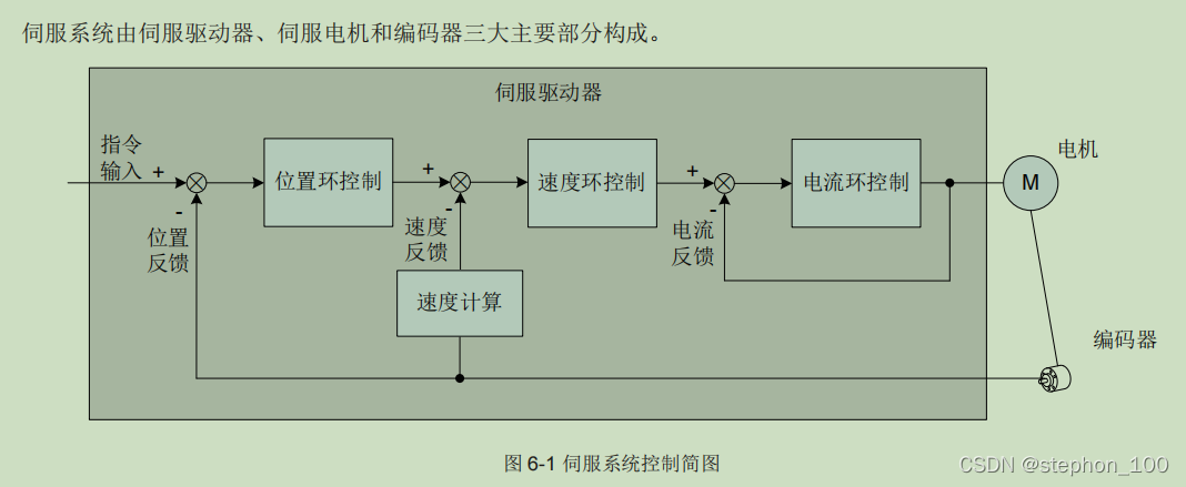
# 摘要
本文全面介绍了伺服驱动器的故障排查艺术,从基础理论到实际应用,详细阐述了伺服驱动器的工作原理、结构与功能以及信号处理机
GX28E01散热解决方案:保障长期稳定运行,让你的设备不再发热
# 摘要
本文针对GX28E01散热问题的严峻性进行了详细探讨。首先,文章从散热理论基础出发,深入介绍了热力学原理及其在散热中的应用,并分析了散热材料与散热器设计的重要性。接着,探讨了硬件和软件层面的散热优化策略,并通过案例分析展示了这些策略在实际中的应用效果。文章进一步探讨了创新的散热技术,如相变冷却技术和主动冷却系统的集成,并展望了散热技术与热管理的未来发展趋势。最后,分析了散热解决方案的经济效益,并探讨了散
无缝集成秘籍:实现UL-kawasaki机器人与PROFINET的完美连接

# 摘要
本文综合介绍了UL-kawasaki机器人与PROFINET通信技术的基础知识、理论解析、实践操作、案例分析以及进阶技巧。首先概述了PROFINET技术原理及其
PDMS设备建模准确度提升:确保设计合规性的5大步骤

# 摘要
本文探讨了PDMS设备建模与设计合规性的基础,深入分析了建模准确度的定义及其与合规性的关系,以及影响PDMS建模准确度的多个因素,包括数据输入质量、建模软件特性和设计者技能等。文章接着提出了确保PDMS建模准确度的策略,包括数据准备、验证流程和最佳建模实践。进一步,本文探讨了PDMS建模准确度的评估方法,涉及内部和外部评估
立即掌握!Aurora 64B-66B v11.2时钟优化与复位策略

# 摘要
本文全面介绍了Aurora 64B/66B的时钟系统架构及其优化策略。首先对Aurora 64B/66B进行简介,然后深入探讨了时钟优化的基础理论,包括时钟域、同步机制和时
掌握CAN协议:10个实用技巧快速提升通信效率
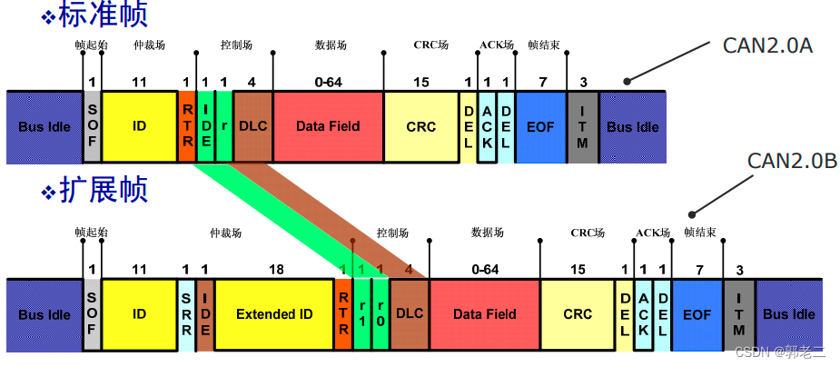
# 摘要
本论文全面介绍了CAN协议的基础原理、硬件选择与配置、软件配置与开发、故障诊断与维护以及在不同领域的应用案例。首先,概述了CAN协议的基本概念和工作原理,然后详细探讨了在选择CAN控制器和收发器、设计网络拓扑结构、连接硬件时应考虑的关键因素以及故障排除技巧。接着,论文重点讨论了软件配置,包括CAN协议栈的选择与配置、消息过滤策略和性能优化。此外,本研究还提供了故障诊断与维护的基
【金字塔构建秘籍】:专家解读GDAL中影像处理速度的极致优化

# 摘要
本文系统地介绍了GDAL影像处理的基础知识、关键概念、实践操作、高级优化技术以及性能评估与调优技巧。文章首先概述了GDAL库的功能和优势,随后深入探讨了影像处理速度优化的理论基础,包括时间复杂度、空间复杂度和多线程并行计算原理,以及GPU硬件加速的应用。在实践操作章节,文章分析了影像格式优化、缓冲区与瓦片技术的应用以及成功案例研究。高级优化技术与工具章节则讨论了分割与融合技术
电子技术期末考试:掌握这8个复习重点,轻松应对考试
# 摘要
本文全面覆盖电子技术期末考试的重要主题和概念,从模拟电子技术到数字电子技术,再到信号与系统理论基础,以及电子技术实验技能的培养。首先介绍了模拟电子技术的核心概念,包括放大电路、振荡器与调制解调技术、滤波器设计。随后,转向数字电子技术的基础知识,如逻辑门电路、计数器与寄存器设计、时序逻辑电路分析。此外,文章还探讨了信号与系统理论基础,涵盖信号分类、线性时不变系统特性、频谱分析与变换。最后,对电子技术实验技能进行了详细阐述,包括电路搭建与测试、元件选型与应用、实验报告撰写与分析。通过对这些主题的深入学习,学生可以充分准备期末考试,并为未来的电子工程项目打下坚实的基础。
# 关键字
模拟
资源上传下载、课程学习等过程中有任何疑问或建议,欢迎提出宝贵意见哦~我们会及时处理!
点击此处反馈


专栏目录
最低0.47元/天 解锁专栏
买1年送3月
百万级
高质量VIP文章无限畅学
千万级
优质资源任意下载
C知道
免费提问 ( 生成式Al产品 )