
ARASARATNAM AND HAYKIN: CUBATURE KALMAN FILTERS 1257
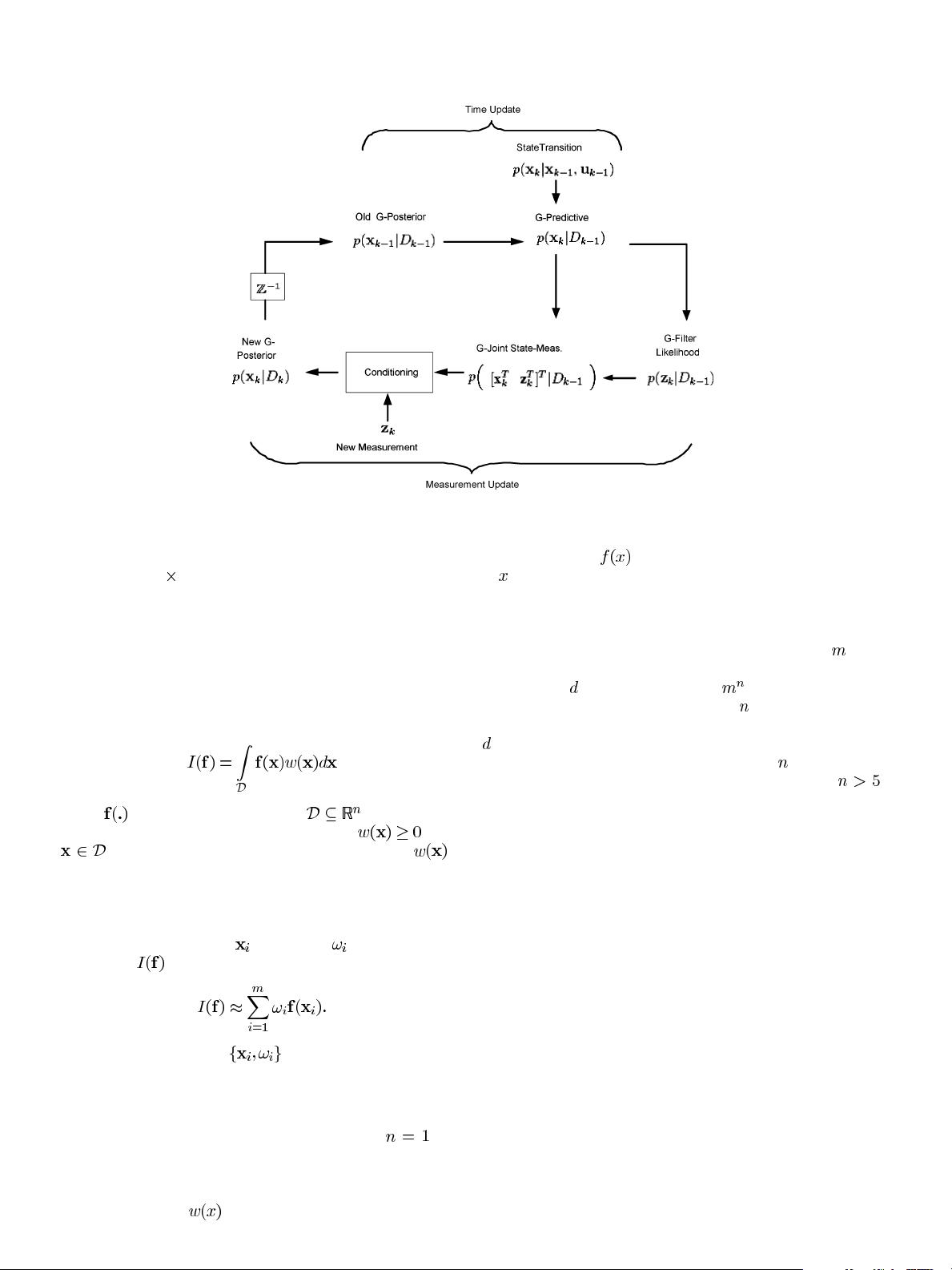
Fig. 2. Signal-flow diagram of the recursive Bayesian filter under the Gaussian assumption, where “G-” stands for “Gaussian-.”
weighted integrals whose integrands are all of the form non-
linear function
Gaussian density that are present in (10),
(11), (13), (14) and (16). The next section describes numerical
integration methods to compute multi-dimensional weighted
integrals.
III. R
EVIEW ON NUMERICAL METHODS
FOR
MOMENT INTEGRALS
Consider a multi-dimensional weighted integral of the form
(21)
where
is some arbitrary function, is the region of
integration, and the known weighting function
for all
. In a Gaussian-weighted integral, for example, is
a Gaussian density and satisfies the nonnegativity condition in
the entire region. If the solution to the above integral (21) is dif-
ficult to obtain, we may seek numerical integration methods to
compute it. The basic task of numerically computing the integral
(21) is to find a set of points
and weights that approximates
the integral
by a weighted sum of function evaluations
(22)
The methods used to find
can be divided into product
rules and non-product rules, as described next.
A. Product Rules
For the simplest one-dimensional case (that is,
), we
may apply the quadrature rule to compute the integral (21)
numerically [21], [22]. In the context of the Bayesian filter,
we mention the Gauss-Hermite quadrature rule; when the
weighting function
is in the form of a Gaussian density
and the integrand
is well approximated by a polynomial
in
, the Gauss-Hermite quadrature rule is used to compute the
Gaussian-weighted integral efficiently [12].
The quadrature rule may be extended to compute multi-
dimensional integrals by successively applying it in a tensor-
product of one-dimensional integrals. Consider an
-point
per dimension quadrature rule that is exact for polynomials of
degree up to
. We set up a grid of points for functional
evaluations and numerically compute an
-dimensional integral
while retaining the accuracy for polynomials of degree up to
only. Hence, the computational complexity of the product
quadrature rule increases exponentially with
, and therefore
suffers from the curse of dimensionality. Typically for
,
the product Gauss-Hermite quadrature rule is not a reasonable
choice to approximate a recursive optimal Bayesian filter.
B. Non-Product Rules
To mitigate the curse of dimensionality issue in the product
rules, we may seek non-product rules for integrals of arbitrary
dimensions by choosing points directly from the domain of in-
tegration [18], [23]. Some of the well-known non-product rules
include randomized Monte Carlo methods [4], quasi-Monte
Carlo methods [24], [25], lattice rules [26] and sparse grids
[27]–[29]. The randomized Monte Carlo methods evaluate the
integration using a set of equally-weighted sample points drawn
randomly, whereas in quasi-Monte Carlo methods and lattice
rules the points are generated from a unit hyper-cube region
using deterministically defined mechanisms. On the other
hand, the sparse grids based on Smolyak formula in principle,
combine a quadrature (univariate) routine for high-dimen-
sional integrals more sophisticatedly; they detect important
dimensions automatically and place more grid points there.
Although the non-product methods mentioned here are pow-
erful numerical integration tools to compute a given integral
with a prescribed accuracy, they do suffer from the curse of
dimensionality to certain extent [30].
剩余15页未读,继续阅读

钢蛋儿(顺利毕业)
- 粉丝: 304
- 资源: 10
 我的内容管理
展开
我的内容管理
展开


最新资源
- 多模态联合稀疏表示在视频目标跟踪中的应用
- Kubernetes资源管控与Gardener开源软件实践解析
- MPI集群监控与负载平衡策略
- 自动化PHP安全漏洞检测:静态代码分析与数据流方法
- 青苔数据CEO程永:技术生态与阿里云开放创新
- 制造业转型: HyperX引领企业上云策略
- 赵维五分享:航空工业电子采购上云实战与运维策略
- 单片机控制的LED点阵显示屏设计及其实现
- 驻云科技李俊涛:AI驱动的云上服务新趋势与挑战
- 6LoWPAN物联网边界路由器:设计与实现
- 猩便利工程师仲小玉:Terraform云资源管理最佳实践与团队协作
- 类差分度改进的互信息特征选择提升文本分类性能
- VERITAS与阿里云合作的混合云转型与数据保护方案
- 云制造中的生产线仿真模型设计与虚拟化研究
- 汪洋在PostgresChina2018分享:高可用 PostgreSQL 工具与架构设计
- 2018 PostgresChina大会:阿里云时空引擎Ganos在PostgreSQL中的创新应用与多模型存储
资源上传下载、课程学习等过程中有任何疑问或建议,欢迎提出宝贵意见哦~我们会及时处理!
点击此处反馈


