[Signal Detection and Classification in MATLAB]: How to Identify Patterns in Signals
发布时间: 2024-09-14 10:56:34 阅读量: 41 订阅数: 49 

EEG ANALYSIS AND CLASSIFICATION:“Electroencephalography (EEG) Signal Enhancement and Analysis”-matlab开发
# [MATLAB Signal Detection and Classification]: How to Identify Patterns in Signals
## 1.1 The Importance of Signal Processing in Modern Technology
In today's rapidly developing field of information technology, signal processing, as a fundamental discipline, plays a crucial role in various domains such as communications, radar, and biomedical engineering. At its core, it involves analyzing, enhancing, filtering, compressing, and other operations on signals using mathematical and algorithmic means to extract information more accurately.
## 1.2 The Role of MATLAB in Signal Processing
MATLAB (an abbreviation for Matrix Laboratory) is a high-performance numerical computing environment and fourth-generation programming language widely used in the field of signal processing. It offers a rich set of signal processing toolboxes, enabling researchers and engineers to perform complex signal processing tasks with ease, including signal generation, analysis, filtering, and pattern recognition.
## 1.3 Overview of the Chapter Content
This chapter will first introduce the basic concepts of signal processing and MATLAB's application background in the field. Following that, we will delve into key topics such as signal detection, signal pattern recognition, and MATLAB implementation. By studying this chapter, readers will gain an initial understanding of MATLAB's signal processing applications and lay a solid foundation for further in-depth learning.
# 2. Fundamental Theory of Signal Detection
### 2.1 Basic Concepts of Signals
#### 2.1.1 Definition and Classification of Signals
In signal processing, a signal can be defined as a physical quantity that varies with time. It can carry information and is used for communication, data transmission, and various measurement processes. According to their physical characteristics, signals can be classified as analog signals and digital signals. Analog signals are continuous in both time and amplitude, such as sound and temperature changes. Digital signals, on the other hand, are discrete and represented by finite discrete values. They are sampled and quantized in both time and amplitude, with common digital signals being digital audio files and digital images.
Signals can also be classified based on whether they change over time. If a signal's characteristics do not change over time, it is non-time-varying. Time-varying signals are those that change with time, such as modulated signals.
Furthermore, signals can be classified according to their statistical characteristics. If all statistical characteristics of a signal, such as mean and variance, remain unchanged throughout the observation period, it is called a stationary signal. Conversely, if these statistical characteristics change over time, it is called a non-stationary signal.
#### 2.1.2 Time-Domain and Frequency-Domain Characteristics of Signals
In the time domain, signals are directly represented as a function of time. For example, sound wave signals can be represented as a curve of sound pressure varying with time. Time-domain analysis mainly focuses on the variation规律 of signals over time, such as signal amplitude, periodicity, and phase.
Frequency-domain analysis involves converting signals from the time domain to the frequency domain to facilitate the analysis of signal frequency components. This is usually achieved through Fourier Transform. In the frequency domain, signals are represented as a superposition of different frequency components, each with a specific amplitude and phase. Frequency-domain analysis can help us identify the main frequency components of a signal, its bandwidth, and the noise components.
### 2.2 Mathematical Foundations of Signal Detection
#### 2.2.1 Fourier Transform and Spectral Analysis
The Fourier Transform is a mathematical tool that converts time-domain signals into frequency-domain signals, revealing the time-domain signal's representation in the frequency domain. The Fourier Transform for continuous-time signals is defined as follows:
```math
F(\omega) = \int_{-\infty}^{\infty} f(t) e^{-j\omega t} dt
```
Where `F(ω)` is the Fourier Transform of the signal `f(t)`, `ω` is the angular frequency, and `j` is the imaginary unit.
The Fourier Transform for discrete-time signals is:
```math
F(k) = \sum_{n=0}^{N-1} f(n) e^{-j\frac{2\pi}{N}kn}
```
Where `F(k)` is the Discrete Fourier Transform (DFT) of the signal `f(n)`, and `N` is the number of sampling points.
Spectral analysis utilizes Fourier Transform to analyze the frequency components of a signal, which is crucial in signal detection. By analyzing the signal's spectrum, we can identify the main frequency components of a signal, which may be generated by the signal source or may be noise-induced.
#### 2.2.2 Wavelet Transform and Time-Frequency Analysis
Compared to the Fourier Transform, the wavelet transform provides a joint time-frequency analysis, making it particularly suitable for analyzing non-stationary signals. The wavelet transform projects the signal onto a series of wavelet functions obtained through scaling and translation transformations. The basic wavelet function (mother wavelet) is of finite support in the time domain and usually has oscillatory characteristics.
The wavelet transform can be represented as:
```math
W(a,b) = \frac{1}{\sqrt{|a|}} \int_{-\infty}^{\infty} f(t) \psi \left(\frac{t-b}{a}\right) dt
```
Where `a` is the scaling parameter, `b` is the translation parameter, and `ψ(t)` is the mother wavelet function.
The wavelet transform can provide a local time-frequency representation of signals, i.e., it can display the frequency characteristics of signals at different times. This is extremely useful for detecting and analyzing signals that change in both time and frequency.
### 2.3 The Impact of Noise on Signal Detection
#### 2.3.1 Types and Characteristics of Noise
In signal processing, noise generally refers to the unwanted, random variations in a signal. Noise can be classified as additive noise and multiplicative noise. Additive noise is directly superimposed on the signal and is independent of the signal's amplitude. Multiplicative noise, on the other hand, is noise related to the signal amplitude, such as quantization noise.
Types of noise include, but are not limited to: white noise, thermal noise, shot noise, 1/f noise, etc. White noise has a flat power spectral density, meaning the power is equal at all frequencies. Thermal noise is a type of random noise that originates from the electronic noise in resistors or other electronic components. Shot noise is due to the random arrival or departure of charge carriers at a point. 1/f noise, also known as flicker noise, has a power spectral density inversely proportional to the frequency.
The impact of noise on signal detection and signal quality is significant; it can obscure the useful parts of a signal, leading to loss of information and misjudgment.
#### 2.3.2 Methods and Strategies for Signal Denoising
Signal denoising is the process of reducing or eliminating noise from a signal, with the aim of improving signal quality and restoring useful information. There are many methods of denoising, including linear filters and non-linear filters.
Linear filters commonly used include the mean filter and the Gaussian filter. The mean filter reduces noise by calculating the average of a set of neighboring signal values, while the Gaussian filter uses the weights of a Gaussian function to calculate the average.
Non-linear filters include the median filter and the bilateral filter. The median filter removes noise by taking the median of a set of neighboring values, while the bilateral filter considers both the brightness and spatial distance information of neighboring pixels, removing noise while preserving edge information.
In MATLAB, the built-in function `filter` can be used to implement linear filtering, and `medfilt2` can be used for median filtering. For example:
```matlab
% Assuming y is a noisy signal and h is a filter
y_filtered = filter(h, 1, y); % Linear filtering
y_median = medfilt2(y); % Median filtering
```
In practical applications, choosing the appropriate denoising method requires considering the characteristics of the signal and noise. For example, if a signal contains sharp edges, a median filter is usually more effective than a mean filter because it can better preserve edge information.
Signal denoising is an important aspect of signal processing. Different denoising strategies and techniques are suitable for different situations. Therefore, before performing signal detection and analysis, it is crucial to accurately assess the nature of the noise and choose an appropriate denoising method.
# 3. MATLAB Signal Detection Practice
## 3.1 MATLAB Signal Generation and Simulation
### 3.1.1 Methods for Generating Basic Signals
Generating basic signals in MATLAB is the starting point for signal processing, including sine waves, square waves, impulse signals, etc. MATLAB provides a series of functions, such as `sin`, `square`, and `impulse`, for generating these basic signals.
The following is an example code for generating a 100Hz sine wave, which is sampled 1000 times in 1 second:
```matlab
Fs = 1000; % Sampling frequency
t = 0:1/Fs:1-1/Fs; % Time vector
f = 100; % Signal frequency
y = sin(2*pi*f*t); % Generating a sine wave
```
This code first defines the sampling frequency `Fs`, then creates a time vector `t`, the length of which and the number of sampling points are determined by `Fs`. The variable `f` is set to 100Hz, representing the signal's frequency. Finally, a sine function generates the desired frequency sine wave.
### 3.1.2 Techniques for Constructing Complex Signals
Complex signals are typically composed of combinations of basic signals, such as modulated signals. In MATLAB, more complex signal models can be constructed by combining basic signals through mathematical operations. For example, an amplitude-modulated (AM) signal can be constructed as follows:
```matlab
Ac = 1; % Carrier amplitude
fc = 500; % Carrier frequency
fm = 50; % Information signal frequency
m = 0.5; % Modulation index
t = 0:1e-5:0.01-1e-5; % Time vector
% Generating carrier signal and modulating signal
carrier = Ac * sin(2*pi*fc*t);
message = sin(2*pi*fm*t);
% Generating AM signal
am_signal = (1+m*message) .* carrier;
% Plotting the AM signal
figure;
plot(t, am_signal);
title('Amplitude Modulated Signal');
xlabel('Time (seconds)');
ylabel('Amplitude');
```
In the above code, `Ac`, `fc`, and `fm` define the amplitude and frequency of the carrier and information signals, respectively, and `m` is the modulation index. By multiplying the information signal and the car

 百万级
高质量VIP文章无限畅学
百万级
高质量VIP文章无限畅学
 千万级
优质资源任意下载
千万级
优质资源任意下载
 C知道
免费提问 ( 生成式Al产品 )
C知道
免费提问 ( 生成式Al产品 )
0
0
相关推荐

专栏目录
最低0.47元/天 解锁专栏
买1年送3月
百万级
高质量VIP文章无限畅学
千万级
优质资源任意下载
C知道
免费提问 ( 生成式Al产品 )
最新推荐
扇形菜单高级应用

# 摘要
扇形菜单作为一种创新的用户界面设计方式,近年来在多个应用领域中显示出其独特优势。本文概述了扇形菜单设计的基本概念和理论基础,深入探讨了其用户交互设计原则和布局算法,并介绍了其在移动端、Web应用和数据可视化中的应用案例
C++ Builder高级特性揭秘:探索模板、STL与泛型编程

# 摘要
本文系统性地介绍了C++ Builder的开发环境设置、模板编程、标准模板库(STL)以及泛型编程的实践与技巧。首先,文章提供了C++ Builder的简介和开发环境的配置指导。接着,深入探讨了C++模板编程的基础知识和高级特性,包括模板的特化、非类型模板参数以及模板
【深入PID调节器】:掌握自动控制原理,实现系统性能最大化

# 摘要
PID调节器是一种广泛应用于工业控制系统中的反馈控制器,它通过比例(P)、积分(I)和微分(D)三种控制作用的组合来调节系统的输出,以实现对被控对象的精确控制。本文详细阐述了PID调节器的概念、组成以及工作原理,并深入探讨了PID参数调整的多种方法和技巧。通过应用实例分析,本文展示了PID调节器在工业过程控制中的实际应用,并讨
【Delphi进阶高手】:动态更新百分比进度条的5个最佳实践

# 摘要
本文针对动态更新进度条在软件开发中的应用进行了深入研究。首先,概述了进度条的基础知识,然后详细分析了在Delphi环境下进度条组件的实现原理、动态更新机制以及多线程同步技术。进一步,文章探讨了数据处理、用户界面响应性优化和状态视觉呈现的实践技巧,并提出了进度
【TongWeb7架构深度剖析】:架构原理与组件功能全面详解
# 摘要
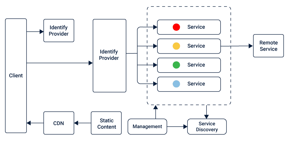
TongWeb7作为一个复杂的网络应用服务器,其架构设计、核心组件解析、性能优化、安全性机制以及扩展性讨论是本文的主要内容。本文首先对TongWeb7的架构进行了概述,然后详细分析了其核心中间件组件的功能与特点,接着探讨了如何优化性能监控与分析、负载均衡、缓存策略等方面,以及安全性机制中的认证授权、数据加密和安全策略实施。最后,本文展望
【S参数秘籍解锁】:掌握驻波比与S参数的终极关系
# 摘要
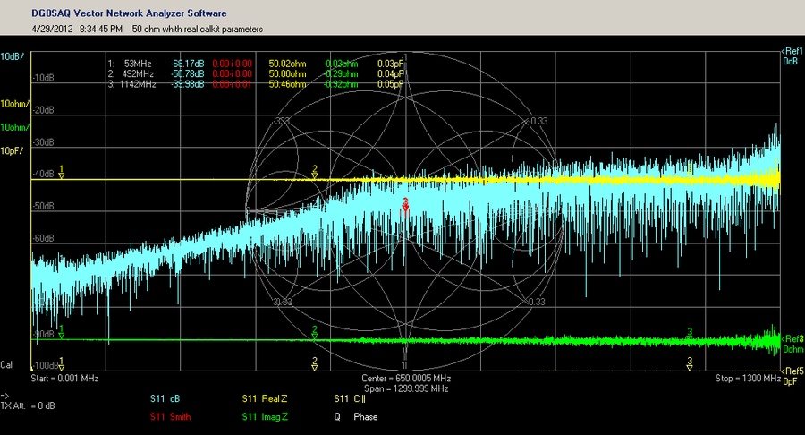
本论文详细阐述了驻波比与S参数的基础理论及其在微波网络中的应用,深入解析了S参数的物理意义、特性、计算方法以及在电路设计中的实践应用。通过分析S参数矩阵的构建原理、测量技术及仿真验证,探讨了S参数在放大器、滤波器设计及阻抗匹配中的重要性。同时,本文还介绍了驻波比的测量、优化策略及其与S参数的互动关系。最后,论文探讨了S参数分析工具的使用、高级分析技巧,并展望
【嵌入式系统功耗优化】:JESD209-5B的终极应用技巧
# 摘要
本文首先概述了嵌入式系统功耗优化的基本情况,随后深入解析了JESD209-5B标准,重点探讨了该标准的框架、核心规范、低功耗技术及实现细节。接着,本文奠定了功耗优化的理论基础,包括功耗的来源、分类、测量技术以及系统级功耗优化理论。进一步,本文通过实践案例深入分析了针对JESD209-5B标准的硬件和软件优化实践,以及不同应用场景下的功耗优化分析。最后,展望了未来嵌入式系统功耗优化的趋势,包括新兴技术的应用、JESD209-5B标准的发展以及绿色计算与可持续发展的结合,探讨了这些因素如何对未来的功耗优化技术产生影响。
# 关键字
嵌入式系统;功耗优化;JESD209-5B标准;低功耗
ODU flex接口的全面解析:如何在现代网络中最大化其潜力
# 摘要
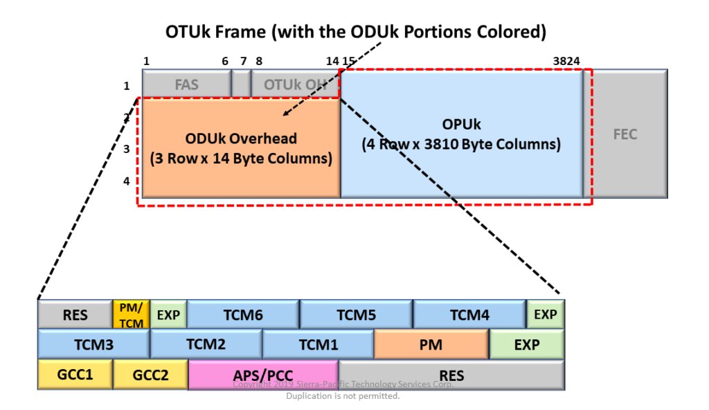
ODU flex接口作为一种高度灵活且可扩展的光传输技术,已经成为现代网络架构优化和电信网络升级的重要组成部分。本文首先概述了ODU flex接口的基本概念和物理层特征,紧接着深入分析了其协议栈和同步机制,揭示了其在数据中心、电信网络、广域网及光纤网络中的应用优势和性能特点。文章进一步
如何最大化先锋SC-LX59的潜力
# 摘要
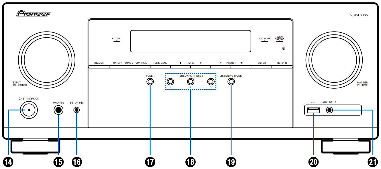
先锋SC-LX59作为一款高端家庭影院接收器,其在音视频性能、用户体验、网络功能和扩展性方面均展现出巨大的潜力。本文首先概述了SC-LX59的基本特点和市场潜力,随后深入探讨了其设置与配置的最佳实践,包括用户界面的个性化和音画效果的调整,连接选项与设备兼容性,以及系统性能的调校。第三章着重于先锋SC-LX59在家庭影院中的应用,特别强调了音视频极致体验、智能家居集成和流媒体服务的充分利用。在高
资源上传下载、课程学习等过程中有任何疑问或建议,欢迎提出宝贵意见哦~我们会及时处理!
点击此处反馈


专栏目录
最低0.47元/天 解锁专栏
买1年送3月
百万级
高质量VIP文章无限畅学
千万级
优质资源任意下载
C知道
免费提问 ( 生成式Al产品 )