Signal Decomposition and Reconstruction in MATLAB: Application of EMD and PCA
发布时间: 2024-09-14 11:06:18 阅读量: 39 订阅数: 49 
# Signal Decomposition and Reconstruction in MATLAB: Applications of EMD and PCA
## 1. Basic Concepts of Signal Processing and Decomposition
In the field of modern information technology, signal processing and decomposition are core technologies for understanding and utilizing signals. Signal processing involves a series of methods used to extract useful information from observational data, while signal decomposition involves breaking down complex signals into more manageable components for analysis. Understanding the fundamental attributes of signals, such as frequency, amplitude, and phase, is the basis for effective analysis. This chapter will introduce the basic concepts of signal processing and decomposition, laying a solid foundation for an in-depth exploration of Empirical Mode Decomposition (EMD) and Principal Component Analysis (PCA) in subsequent chapters. We will start with the basic properties of signals, gradually unfolding the concepts to help readers gain a comprehensive understanding of signal analysis.
## 2. Empirical Mode Decomposition (EMD) Theory and Practice
Empirical Mode Decomposition (EMD) is a method for processing nonlinear and non-stationary signals. It decomposes complex signals into a series of Intrinsic Mode Functions (IMFs), which can be linear or nonlinear but have clear physical significance. EMD holds an important position in the field of signal processing and is fundamental to understanding the content of subsequent chapters.
### 2.1 Theoretical Basis of the EMD Method
#### 2.1.1 Instantaneous Frequency and Hilbert Transform
The concept of instantaneous frequency is key to understanding EMD. In traditional Fourier transforms, frequency is considered constant, which is appropriate for processing stationary signals but inadequate for non-stationary signals. The introduction of instantaneous frequency allows frequency to vary with time, providing a theoretical basis for EMD.
The Hilbert transform is a common mathematical tool for obtaining instantaneous frequency. It converts a signal into an analytic signal, thereby obtaining instantaneous amplitude and instantaneous frequency. The Hilbert transform is often used in signal processing, such as in AM and FM modulation/demodulation, and in EMD to determine the instantaneous frequency of IMFs.
#### 2.1.2 Generation of Intrinsic Mode Functions (IMFs)
IMFs are the core concept in the EMD process, referring to the physical meaningful oscillatory modes within a signal. An ideal IMF must satisfy two conditions: at any point, the number of local maxima and minima must be equal or differ by at most one; at any point, the mean value of the upper envelope defined by local maxima and the lower envelope defined by local minima must be zero.
The generation of IMFs is achieved through an iterative algorithm known as the "sifting" process. This process iterates until the conditions for an IMF are met. Each iteration extracts an IMF component from the original signal.
### 2.2 Applications of EMD in Signal Decomposition
#### 2.2.1 Decomposition Process and Steps
The EMD decomposition steps are typically as follows:
1. **Initialization:** Identify all maxima and minima in the original signal and construct upper and lower envelope lines.
2. **Sifting Process:** Calculate the average of the upper and lower envelope lines and subtract it from the original signal to obtain a residual.
3. **Iteration:** Treat the residual as a new signal and repeat the above process until the definition of an IMF is satisfied.
4. **Extracting IMFs:** Each iteration produces an IMF component, which is sequentially separated from the original signal, ultimately yielding IMFs and a residual trend term.
#### 2.2.2 Physical Meaning of Decomposition Results
The decomposition results of EMD describe the local characteristics of the original signal at different time scales. Each IMF represents a basic oscillatory mode in the signal, with its frequency varying over time, revealing the dynamic characteristics of the signal at different time scales.
The physical meaning of the decomposition results is mainly reflected in the ability to more accurately analyze non-stationary signals. For example, EMD can identify sudden changes, trend changes, and periodic changes in the signal, which is difficult for traditional linear analysis methods to achieve.
### 2.3 Limitations of EMD and Improvement Methods
#### 2.3.1 End Effect and Envelope Fitting
In the EMD decomposition process, the end effect is an unavoidable issue. The end effect mainly manifests as interference to the IMFs near the boundaries, which can lead to inaccurate decomposition results. One improvement method is to use reflective boundary conditions, that is, by mirroring the endpoints of the original signal to extend the signal, thereby reducing the end effect.
The accuracy of envelope fitting also directly affects the effectiveness of EMD. Typically, cubic spline interpolation is used to fit the envelope, which requires careful parameter adjustment to ensure the quality of the fit.
#### 2.3.2 Optimization Strategies from Theory to Practical Application
When applying EMD to practical problems, the algorithm needs to be adjusted and optimized based on specific conditions. For example, for signals with a high level of noise, filtering can be performed first to reduce the impact of noise; for signals that require analysis of a specific frequency range, prescreening stop conditions can be defined to obtain IMFs at specific scales.
Optimization strategies also involve selecting appropriate stopping criteria to avoid over-decomposition, resulting in IMFs losing their physical significance. In practical applications, continuous trials and verifications are needed to find the best decomposition scheme.
## 3. Foundations and Implementation of Principal Component Analysis (PCA)
## 3.1 Mathematical Principles of PCA
### 3.1.1 Covariance Matrix and Eigenvalue Decomposition
Principal Component Analysis (PCA) is a widely used technique for dimensionality reduction. It transforms the original data into a new set of linearly uncorrelated coordinates through a linear transformation, where the directions correspond to the eigenvectors of the data's covariance matrix. In this new space, the first principal component has the largest variance, each subsequent component has the largest remaining variance, and each is orthogonal to all preceding components.
The covariance matrix of a dataset describes the correlation between variables within the dataset. Specifically, for a dataset $X$ containing $m$ samples, each with $n$ dimensions, its covariance matrix $C$ can be represented by the following formula:
C = \frac{1}{m-1} X^T X
where $X^T$ represents the transpose of the matrix $X$. The resulting covariance matrix is an $n \times n$ symmetric matrix.
### 3.1.2 Extraction and Interpretation of Principal Components
Next, PCA extracts the principal components of the data through eigenvalue decomposition. The process of eigenvalue decomposition is as follows:
1. Calculate the eigenvalues $\lambda_i$ and corresponding eigenvectors $e_i$ of the covariance matrix $C$.
2. Sort the eigenvalues in descending order.
3. The eigenvectors form new basis vectors, which are arranged into a matrix $P$ for transforming the original data.
Projecting the original dataset $X$ onto the eigenvectors gives a new dataset $Y$:
Y = X P
where $Y$ is the representation of the original data in the new feature space, its dimension is $m \times n$, and usually, the first $k$ eigenvectors ($k < n$) can explain most of the data variance.
## 3.2 Applications of PCA in Data Dimensionality Reduction
### 3.2.1 Data Preprocessing and Standardization
Before using PCA, data often needs to be preprocessed and standa***mon methods include centering and scaling:
- **Centering:** Subtract the mean of each feature so that the data's center is at the origin.
- **Scaling:** Normalize the variance of each feature to 1, giving each feature the same scale.
The standardization formula is as follows:
x_{\text{normalized}} = \frac{x - \mu}{\sigma}
where $x$ is the original feature value, $\mu$ is the mean of the feature, and $\sigma$ is the standard deviation of the feature.
### 3.2.2 Evaluation and Selection of Dimensionality Reduction Effects
A common indicator for evaluating the effect of dimensionality reduction is the ratio of explained variance, which represents the amount of variance information of the original data contained in each principal component. By accumulating the ratio of explained variance, the number of principal components used can be determined to meet the needs of data compression and explanation. Generally, we select the number of principal components that cumulatively reach a specific threshold (e.g., 95%).
## 3.3 Implementation and Case Analysis of PCA
### 3.3.1 Steps for Implementing PCA in MATLAB
In MATLAB, the built-in function `pca` can be used for PCA analysis. The following are the basic steps for performing PCA analysis in MATLAB:
1. Prepare the dataset `X` and ensure it is in matrix format.
2. Use the `pca` function to perform PCA analysis:
```matlab
[coeff, score, latent] = pca(X);
```
Here, `coeff` is the matrix of eigenvectors, `score` is the transformed data matrix, and `latent` contains the eigenvalues.
3. Analyze the output results, including the explained variance ratio of

 百万级
高质量VIP文章无限畅学
百万级
高质量VIP文章无限畅学
 千万级
优质资源任意下载
千万级
优质资源任意下载
 C知道
免费提问 ( 生成式Al产品 )
C知道
免费提问 ( 生成式Al产品 )
0
0
相关推荐

专栏目录
最低0.47元/天 解锁专栏
买1年送3月
百万级
高质量VIP文章无限畅学
千万级
优质资源任意下载
C知道
免费提问 ( 生成式Al产品 )
最新推荐
AMESim液压仿真秘籍:专家级技巧助你从基础飞跃至顶尖水平

# 摘要
AMESim液压仿真软件是工程师们进行液压系统设计与分析的强大工具,它通过图形化界面简化了模型建立和仿真的流程。本文旨在为用户提供AMESim软件的全面介绍,从基础操作到高级技巧,再到项目实践案例分析,并对未来技术发展趋势进行展望。文中详细说明了AMESim的安装、界面熟悉、基础和高级液压模型的建立,以及如何运行、分析和验证仿真结果。通过探索自定义组件开发、多学科仿真集成以及高级仿真算法的应用,本文
【高频领域挑战】:VCO设计在微波工程中的突破与机遇
# 摘要
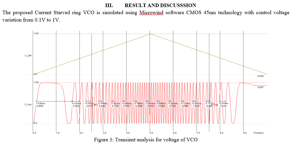
本论文深入探讨了压控振荡器(VCO)的基础理论与核心设计原则,并在微波工程的应用技术中展开详细讨论。通过对VCO工作原理、关键性能指标以及在微波通信系统中的作用进行分析,本文揭示了VCO设计面临的主要挑战,并提出了相应的技术对策,包括频率稳定性提升和噪声性能优化的方法。此外,论文还探讨了VCO设计的实践方法、案例分析和故障诊断策略,最后对VCO设计的创新思路、新技术趋势及未来发展挑战
实现SUN2000数据采集:MODBUS编程实践,数据掌控不二法门
# 摘要
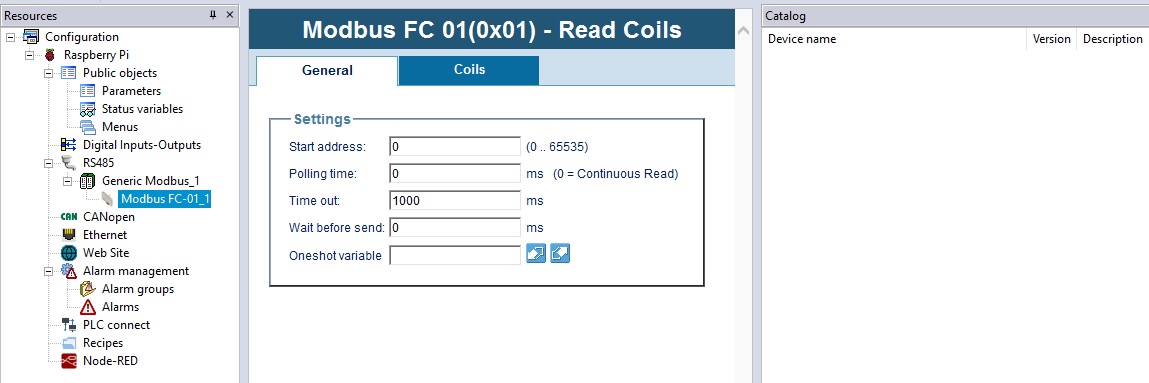
本文系统地介绍了MODBUS协议及其在数据采集中的应用。首先,概述了MODBUS协议的基本原理和数据采集的基础知识。随后,详细解析了MODBUS协议的工作原理、地址和数据模型以及通讯模式,包括RTU和ASCII模式的特性及应用。紧接着,通过Python语言的MODBUS库,展示了MODBUS数据读取和写入的编程实践,提供了具体的实现方法和异常管理策略。本文还结合SUN20
【性能调优秘籍】:深度解析sco506系统安装后的优化策略
# 摘要
本文对sco506系统的性能调优进行了全面的介绍,首先概述了性能调优的基本概念,并对sco506系统的核心组件进行了介绍。深入探讨了核心参数调整、磁盘I/O、网络性能调优等关键性能领域。此外,本文还揭示了高级性能调优技巧,包括CPU资源和内存管理,以及文件系统性能的调整。为确保系统的安全性能,文章详细讨论了安全策略、防火墙与入侵检测系统的配置,以及系统审计与日志管理的优化。最后,本文提供了系统监控与维护的
网络延迟不再难题:实验二中常见问题的快速解决之道
# 摘要
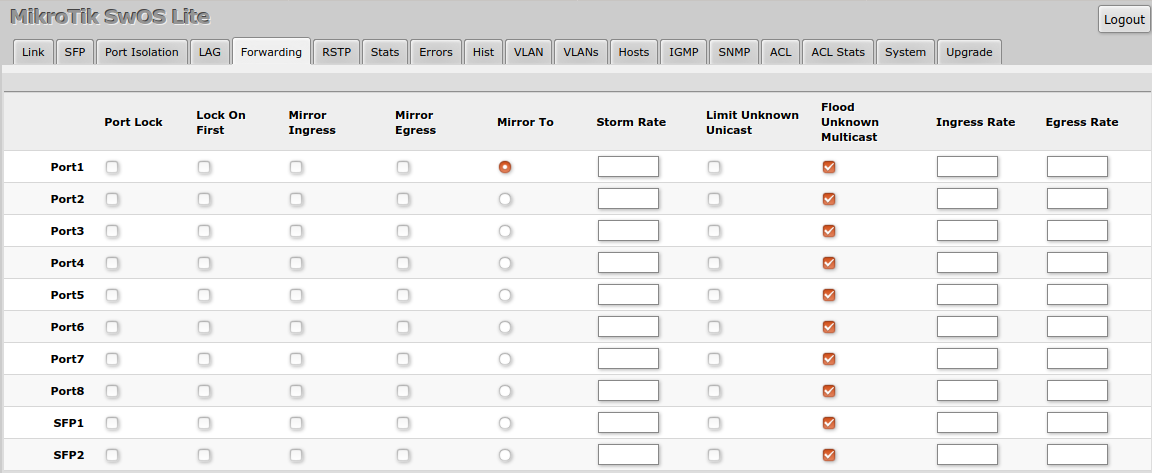
网络延迟是影响网络性能的重要因素,其成因复杂,涉及网络架构、传输协议、硬件设备等多个方面。本文系统分析了网络延迟的成因及其对网络通信的影响,并探讨了网络延迟的测量、监控与优化策略。通过对不同测量工具和监控方法的比较,提出了针对性的网络架构优化方案,包括硬件升级、协议配置调整和资源动态管理等。
期末考试必备:移动互联网商业模式与用户体验设计精讲

# 摘要
移动互联网的迅速发展带动了商业模式的创新,同时用户体验设计的重要性日益凸显。本文首先概述了移动互联网商业模式的基本概念,接着深入探讨用户体验设计的基础,包括用户体验的定义、重要性、用户研究方法和交互设计原则。文章重点分析了移动应用的交互设计和视觉设计原则,并提供了设计实践案例。之后,文章转向移动商业模式的构建与创新,探讨了商业模式框架
【多语言环境编码实践】:在各种语言环境下正确处理UTF-8与GB2312
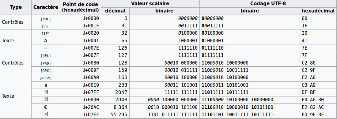
# 摘要
随着全球化的推进和互联网技术的发展,多语言环境下的编码问题变得日益重要。本文首先概述了编码基础与字符集,随后深入探讨了多语言环境所面临的编码挑战,包括字符编码的重要性、编码选择的考量以及编码转换的原则和方法。在此基础上,文章详细介绍了UTF-8和GB2312编码机制,并对两者进行了比较分析。此外,本文还分享了在不同编程语言中处理编码的实践技巧,
【数据库在人事管理系统中的应用】:理论与实践:专业解析
# 摘要
本文探讨了人事管理系统与数据库的紧密关系,分析了数据库设计的基础理论、规范化过程以及性能优化的实践策略。文中详细阐述了人事管理系统的数据库实现,包括表设计、视图、存储过程、触发器和事务处理机制。同时,本研究着重讨论了数据库的安全性问题,提出认证、授权、加密和备份等关键安全策略,以及维护和故障处理的最佳实践。最后,文章展望了人事管理系统的发展趋
【Docker MySQL故障诊断】:三步解决权限被拒难题
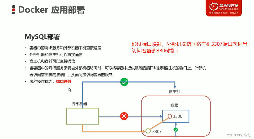
# 摘要
随着容器化技术的广泛应用,Docker已成为管理MySQL数据库的流行方式。本文旨在对Docker环境下MySQL权限问题进行系统的故障诊断概述,阐述了MySQL权限模型的基础理论和在Docker环境下的特殊性。通过理论与实践相结合,提出了诊断权限问题的流程和常见原因分析。本文还详细介绍了如何利用日志文件、配置检查以及命令行工具进行故障定位与修复,并探讨了权限被拒问题的解决策略和预防措施
资源上传下载、课程学习等过程中有任何疑问或建议,欢迎提出宝贵意见哦~我们会及时处理!
点击此处反馈


专栏目录
最低0.47元/天 解锁专栏
买1年送3月
百万级
高质量VIP文章无限畅学
千万级
优质资源任意下载
C知道
免费提问 ( 生成式Al产品 )