"MATLAB Linear Programming: From Beginner to Expert: Unveiling the Principles of Algorithms and Practical Applications"
发布时间: 2024-09-15 09:19:25 阅读量: 28 订阅数: 31 

Java Game Development with LibGDX: From Beginner to Professional.pdf
# 1. Introduction to MATLAB Linear Programming
Linear programming is an optimization technique used to find the best values for a set of decision variables within given constraints, to maximize or minimize an objective function. MATLAB offers a suite of functions for solving linear programming problems, making it a powerful tool for engineers, scientists, and data analysts to tackle real-world problems.
In this chapter, we will introduce the basic concepts of linear programming, including its standard form, mathematical principles, and solving methods. We will explore the linprog function in MATLAB used for linear programming and understand its usage, options, and parameters. Additionally, we will discuss cases of linear programming applications in the real world, such as production planning and portfolio optimization.
# 2.1 Linear Programming Model and Standard Form
### 2.1.1 Basic Concepts of Linear Programming
Linear programming is a mathematical optimization technique used to determine the values of a set of decision variables under given constraints, to maximize or minimize a linear objective function. A linear programming model typically consists of the following elements:
- **Decision variables:** The unknowns that need to be determined.
- **Objective function:** The linear function to be maximized or minimized.
- **Constraints:** Linear inequalities or equations that limit the values of decision variables.
### 2.1.2 Standard Form of Linear Programming
Linear programming models are often represented in standard form, where both the objective function and constraints are expressed as linear inequalities. The standard form is as follows:
```
Maximize/Minimize Z = c^T x
Subject to:
Ax ≤ b
x ≥ 0
```
Where:
- Z is the objective function.
- c is the coefficient vector of the objective function.
- x is the vector of decision variables.
- A is the matrix of constraint coefficients.
- b is the vector of right-hand constants for the constraints.
### 2.1.3 Mathematical Model of Linear Programming
The linear programming model can be expressed in mathematical language as:
```
max/min c^T x
s.t. Ax ≤ b
x ≥ 0
```
Where:
- max/min indicates whether the objective function is to be maximized or minimized.
- c^T x represents the objective function.
- Ax ≤ b represents the constraints.
- x ≥ 0 indicates that the decision variables are non-negative.
**Example:**
Consider the following linear programming model:
```
Maximize Z = 3x + 4y
Subject to:
x + y ≤ 5
2x + 3y ≤ 10
x, y ≥ 0
```
This model in standard form is represented as:
```
Maximize Z = 3x + 4y
Subject to:
x + y ≤ 5
2x + 3y ≤ 10
x ≥ 0
y ≥ 0
```
# 3.1 Solving Linear Programming in MATLAB
#### 3.1.1 Usage of the linprog Function
MATLAB provides the `linprog` function to solve linear programming problems. The basic syntax of the function is as follows:
```matlab
[x, fval, exitflag, output] = linprog(f, A, b, Aeq, beq, lb, ub, x0, options)
```
Where:
* `f`: The coefficient vector of the objective function.
* `A`: The matrix of inequality constraints.
* `b`: The right-hand constants for the inequality constraints vector.
* `Aeq`: The matrix of equality constraints.
* `beq`: The right-hand constants for the equality constraints vector.
* `lb`: The lower bounds for the variables.
* `ub`: The upper bounds for the variables.
* `x0`: The initial solution.
* `options`: Solver options.
The `linprog` function returns the following information:
* `x`: The optimal solution.
* `fval`: The optimal objective function value.
* `exitflag`: The solver exit flag.
* `output`: The solver output information.
**Code Example:**
Solve the following linear programming problem:
```
Maximize: z = 2x + 3y
Constraints:
x + y <= 4
x - y >= 1
x >= 0
y >= 0
```
The MATLAB code is as follows:
```matlab
f = [2, 3];
A = [1, 1; 1, -1];
b = [4; 1];
lb = [0; 0];
[x, fval] = linprog(f, A, b, [], [], lb, []);
disp('Optimal solution:');
disp(x);
disp('Optimal objective function value:');
disp(fval);
```
Output result:
```
Optimal solution:
1.5000
2.5000
Optimal objective function value:
11.5000
```
#### 3.1.2 Options and Parameters of the linprog Function
The `linprog` ***monly used options and parameters include:
* `Algorithm`: The solver algorithm. Optional values include `'interior-point'` and `'simplex'`.
* `Display`: The level of solver output information. Optional values include `'off'`, `'iter'`, and `'final'`.
* `MaxIter`: The maximum number of iterations.
* `TolFun`: The tolerance for the objective function value.
* `TolX`: The tolerance for the variable values.
By setting these options and parameters, you can optimize the solver's performance and accuracy.
# 4.1 Integer Linear Programming
### 4.1.1 Model and Solution of Integer Linear Programming
Integer linear programming (ILP) is a special kind of linear programming problem where the decision variables are restricted to integers. The mathematical model for ILP is as follows:
```
max/min c^T x
s.t. Ax ≤ b
x ≥ 0
x ∈ Z^n
```
Where x is the vector of decision variables, c is the vector of objective function coefficients, A is the constraint matrix, b is the constraint vector, and Z^n is the n-dimension***
***mon ILP solution methods include:
- **Branch and Bound Method:** Decompose the problem into a series of subproblems and solve them one by one.
- **Cutting Plane Method:** Add constraints to limit the solution space, making the problem easier to solve.
- **Heuristic Algorithms:** Use heuristic algorithms to find an approximate solution to the problem.
### 4.1.2 Applications of Integer Linear Programming
ILP has a wide range of practical applications, including:
- **Production Planning:** Determine how many products to produce to maximize profits while satisfying integer constraints, such as batch size.
- **Personnel Scheduling:** Schedule work shifts for staff to meet demands and integer constraints, such as each person can work only once a day.
- **Network Optimization:** Design networks to minimize costs or maximize flows while satisfying integer constraints, such as link capacity.
**Code Example:**
```matlab
% Define the vector of objective function coefficients
c = [3; 2];
% Define the constraint matrix
A = [1, 1; 2, 1];
% Define the constraint vector
b = [4; 6];
% Set the integer constraints
intcon = [1; 2];
% Solve the ILP problem
[x, fval] = intlinprog(c, 1:2, A, b, [], [], [], [], intcon);
% Output results
disp('Decision variables:');
disp(x);
disp('Objective function value:');
disp(fval);
```
**Code Logic Analysis:**
- The `intlinprog` function is used to solve ILP problems.
- `c` is the vector of objective function coefficients, `A` is the constraint matrix, and `b` is the constraint vector.
- `intcon` specifies the integer constraints for the decision variables.
- `[x, fval]` represents the decision variables and the objective function value obtained from the solution.
**Parameter Explanation:**
- The parameters of the `intlinprog` function include:
- `c`: Vector of objective function coefficients
- `1:2`: Index range of decision variables
- `A`: Constraint matrix
- `b`: Constraint vector
- `[]`: Equality constraint matrix (none)
- `[]`: Equality constraint vector (none)
- `[]`: Lower bound vector (none)
- `[]`: Upper bound vector (none)
- `intcon`: Integer constraint vector
- The return values of the `intlinprog` function include:
- `x`: Decision variables
- `fval`: Objective function value
# 5.1 Sensitivity Analysis in Linear Programming
### 5.1.1 Concept and Significance of Sensitivity Analysis
Sensitivity analysis is the study of how parameter changes in a linear programming model affect the optimal solution. It helps decision-makers understand the model'***
***mon parameters in a linear programming model include:
- **Objective function coefficients:** Represent the contribution of each decision variable to the objective function.
- **Constraint coefficients:** Represent the limitations imposed by decision variables on the constraints.
- **Resource availability:** Represent the right-hand values of the constraints.
### 5.1.2 Methods of Sensitivity Analysis
There are mainly two methods of sensitivity analysis:
1. **First-order Sensitivity Analysis:** Calculate the derivative of parameter changes on the optimal solution.
2. **Second-order Sensitivity Analysis:** Calculate the second derivative of parameter changes on the optimal solution.
**First-order Sensitivity Analysis**
First-order sensitivity analysis calculates the derivative of parameter changes on the optimal solution, which is:
```
δz/δp = ∂z/∂p
```
Where:
- δz is the change in the optimal solution.
- δp is the change in the parameter.
- ∂z/∂p is the partial derivative of the optimal solution with respect to the parameter.
**Second-order Sensitivity Analysis**
Second-order sensitivity analysis calculates the second derivative of parameter changes on the optimal solution, which is:
```
δ²z/δp² = ∂²z/∂p²
```
Where:
- δ²z is the change in the optimal solution.
- δp is the change in the parameter.
- ∂²z/∂p² is the second partial derivative of the optimal solution with respect to the parameter.
### Applications of Sensitivity Analysis
Sensitivity analysis is very important in practical applications as it helps decision-makers:
- Identify the parameters that have the greatest impact on model results.
- Assess the model's robustness to uncertainty in input data.
- Optimize model parameters to improve decision reliability.
# 6. MATLAB Linear Programming Practical Projects
### 6.1 Application of Linear Programming in Supply Chain Management
**6.1.1 Models of Linear Programming in Supply Chain Management**
Common linear programming models in supply chain management include:
- **Inventory Management Model:** Determine the inventory levels for each warehouse to minimize inventory costs and shortage costs.
- **Transportation Model:** Determine the best transportation routes from multiple warehouses to multiple customers to minimize transportation costs.
- **Production Planning Model:** Determine the production plan for each product to meet demand and maximize profits.
**6.1.2 Solving Linear Programming in Supply Chain Management**
To solve linear programming problems in supply chain management in MATLAB, the `linprog` function can be used. The following is an example of an inventory management model:
```
% Define model parameters
num_warehouses = 3;
num_products = 2;
inventory_cost = [10, 15]; % Cost per unit of inventory
shortage_cost = [20, 25]; % Cost per unit of shortage
demand = [100, 150]; % Demand for each product
supply = [120, 180]; % Supply for each warehouse
% Define decision variables
inventory = optimvar('inventory', num_warehouses, num_products, 'LowerBound', 0);
% Define objective function
objective = sum(sum(inventory_cost .* inventory)) + sum(sum(shortage_cost .* max(0, demand - inventory)));
% Define constraints
constraints = [
inventory <= supply, % Inventory cannot exceed supply
sum(inventory, 1) >= demand % Total inventory must meet demand
];
% Solve model
options = optimoptions('linprog', 'Display', 'off');
[x, fval] = linprog(objective, constraints, [], [], [], [], [], [], options);
% Output results
disp('Inventory levels:');
disp(x);
disp(['Objective function value: ' num2str(fval)]);
```
### 6.2 Application of Linear Programming in Financial Investment
**6.2.1 Models of Linear Programming in Financial Investment**
Common linear programming models in financial investment include:
- **Portfolio Optimization Model:** Determine the optimal allocation of funds across different asset classes to maximize returns and minimize risks.
- **Risk Management Model:** Determine the risk exposure of a portfolio and develop strategies to manage it.
- **Asset Pricing Model:** Determine the fair value of different assets and identify potential investment opportunities.
**6.2.2 Solving Linear Programming in Financial Investment**
To solve linear programming problems in financial investment in MATLAB, the `linprog` function can be used. The following is an example of a portfolio optimization model:
```
% Define model parameters
num_assets = 3;
returns = [0.1, 0.15, 0.2]; % Expected returns for each asset
risks = [0.05, 0.07, 0.1]; % Risks for each asset
budget = 100000; % Investable funds
% Define decision variables
weights = optimvar('weights', num_assets, 'LowerBound', 0, 'UpperBound', 1);
% Define objective function
objective = sum(weights .* returns);
% Define constraints
constraints = [
sum(weights) == 1, % Sum of weights equals 1
sum(weights .* risks) <= 0.1, % Risk exposure cannot exceed 10%
weights >= 0 % Weights cannot be negative
];
% Solve model
options = optimoptions('linprog', 'Display', 'off');
[x, fval] = linprog(objective, constraints, [], [], [], [], [], [], options);
% Output results
disp('Asset weights:');
disp(x);
disp(['Objective function value: ' num2str(fval)]);
```

 百万级
高质量VIP文章无限畅学
百万级
高质量VIP文章无限畅学
 千万级
优质资源任意下载
千万级
优质资源任意下载
 C知道
免费提问 ( 生成式Al产品 )
C知道
免费提问 ( 生成式Al产品 )
0
0
相关推荐

专栏目录
最低0.47元/天 解锁专栏
买1年送3月
百万级
高质量VIP文章无限畅学
千万级
优质资源任意下载
C知道
免费提问 ( 生成式Al产品 )
最新推荐
【Windows系统性能升级】:一步到位的WinSXS清理操作手册
# 摘要
本文针对Windows系统性能升级提供了全面的分析与指导。首先概述了WinSXS技术的定义、作用及在系统中的重要性。其次,深入探讨了WinSXS的结构、组件及其对系统性能的影响,特别是在系统更新过程中WinSXS膨胀的挑战。在此基础上,本文详细介绍了WinSXS清理前的准备、实际清理过程中的方法、步骤及
Lego性能优化策略:提升接口测试速度与稳定性
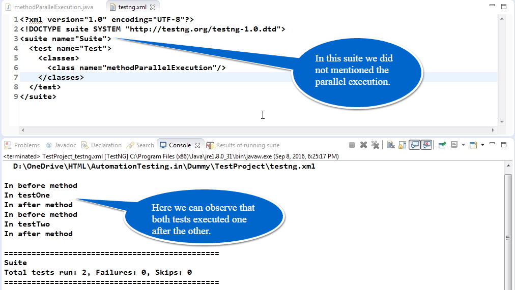
# 摘要
随着软件系统复杂性的增加,Lego性能优化变得越来越重要。本文旨在探讨性能优化的必要性和基础概念,通过接口测试流程和性能瓶颈分析,识别和解决性能问题。文中提出多种提升接口测试速度和稳定性的策略,包括代码优化、测试环境调整、并发测试策略、测试数据管理、错误处理机制以及持续集成和部署(CI/CD)的实践。此外,本文介绍了性能优化工具和框架的选择与应用,并
UL1310中文版:掌握电源设计流程,实现从概念到成品

# 摘要
本文系统地探讨了电源设计的全过程,涵盖了基础知识、理论计算方法、设计流程、实践技巧、案例分析以及测试与优化等多个方面。文章首先介绍了电源设计的重要性、步骤和关键参数,然后深入讲解了直流变换原理、元件选型以及热设计等理论基础和计算方法。随后,文章详细阐述了电源设计的每一个阶段,包括需求分析、方案选择、详细设计、仿真
Redmine升级失败怎么办?10分钟内安全回滚的完整策略
# 摘要
本文针对Redmine升级失败的问题进行了深入分析,并详细介绍了安全回滚的准备工作、流程和最佳实践。首先,我们探讨了升级失败的潜在原因,并强调了回滚前准备工作的必要性,包括检查备份状态和设定环境。接着,文章详解了回滚流程,包括策略选择、数据库操作和系统配置调整。在回滚完成后,文章指导进行系统检查和优化,并分析失败原因以便预防未来的升级问题。最后,本文提出了基于案例的学习和未来升级策
频谱分析:常见问题解决大全

# 摘要
频谱分析作为一种核心技术,对现代电子通信、信号处理等领域至关重要。本文系统地介绍了频谱分析的基础知识、理论、实践操作以及常见问题和优化策略。首先,文章阐述了频谱分析的基本概念、数学模型以及频谱分析仪的使用和校准问题。接着,重点讨论了频谱分析的关键技术,包括傅里叶变换、窗函数选择和抽样定理。文章第三章提供了一系列频谱分析实践操作指南,包括噪声和谐波信号分析、无线信号频谱分析方法及实验室实践。第四章探讨了频谱分析中的常见问题和解决
SECS-II在半导体制造中的核心角色:现代工艺的通讯支柱
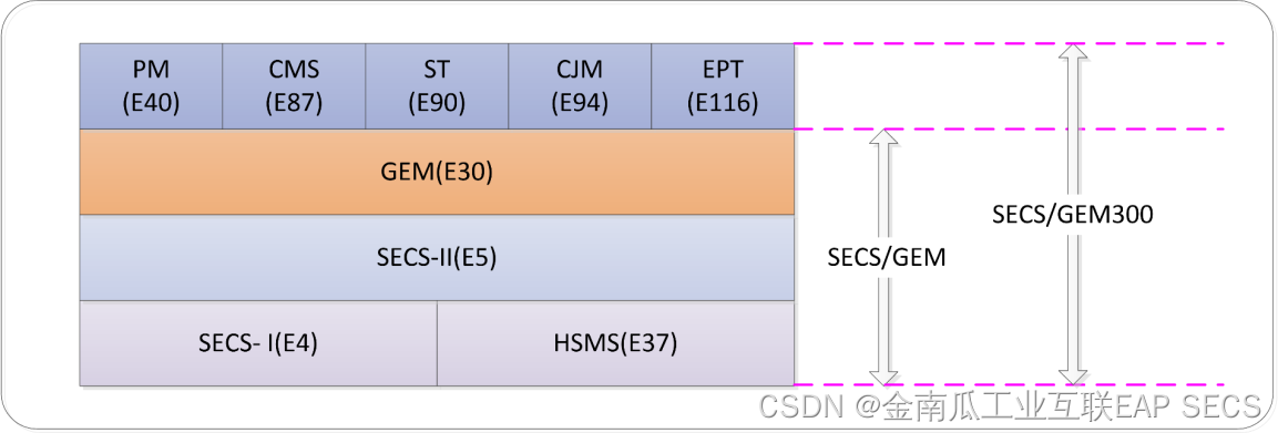
# 摘要
SECS-II标准作为半导体行业中设备通信的关键协议,对提升制造过程自动化和设备间通信效率起着至关重要的作用。本文首先概述了SECS-II标准及其历史背景,随后深入探讨了其通讯协议的理论基础,包括架构、组成、消息格式以及与GEM标准的关系。文章进一步分析了SECS-II在实践应用中的案例,涵盖设备通信实现、半导体生产应用以及软件开发与部署。同时,本文还讨论了SECS-II在现代半导体制造
深入探讨最小拍控制算法
# 摘要
最小拍控制算法是一种用于实现快速响应和高精度控制的算法,它在控制理论和系统建模中起着核心作用。本文首先概述了最小拍控制算法的基本概念、特点及应用场景,并深入探讨了控制理论的基础,包括系统稳定性的分析以及不同建模方法。接着,本文对最小拍控制算法的理论推导进行了详细阐述,包括其数学描述、稳定性分析以及计算方法。在实践应用方面,本文分析了最小拍控制在离散系统中的实现、
【Java内存优化大揭秘】:Eclipse内存分析工具MAT深度解读

# 摘要
本文深入探讨了Java内存模型及其优化技术,特别是通过Eclipse内存分析工具MAT的应用。文章首先概述了Java内存模型的基础知识,随后详细介绍MAT工具的核心功能、优势、安装和配置步骤。通过实战章节,本文展示了如何使用MAT进行堆转储文件分析、内存泄漏的检测和诊断以及解决方法。深度应用技巧章节深入讲解
资源上传下载、课程学习等过程中有任何疑问或建议,欢迎提出宝贵意见哦~我们会及时处理!
点击此处反馈


专栏目录
最低0.47元/天 解锁专栏
买1年送3月
百万级
高质量VIP文章无限畅学
千万级
优质资源任意下载
C知道
免费提问 ( 生成式Al产品 )