【MATLAB Genetic Algorithm: From Beginner to Expert】: A Comprehensive Guide to Master Genetic Algorithms for Practical Application
发布时间: 2024-09-15 03:45:49 阅读量: 72 订阅数: 23 
# From Novice to Expert: A Comprehensive Guide to Genetic Algorithms in MATLAB
## Chapter 1: Fundamentals of Genetic Algorithms
Genetic algorithms are search and optimization algorithms that mimic the principles of natural selection and genetics. They belong to the broader category of evolutionary algorithms. In this chapter, we will explore the basic concepts of genetic algorithms, including their origin, core ideas, and the fundamental process of solving problems. Genetic algorithms use a mechanism of "survival of the fittest and elimination of the unfit" to find the optimal solutions to problems, emulating the biological evolutionary process.
### The Origin and Development of Genetic Algorithms
The concept of genetic algorithms was first proposed by Professor John Holland in the 1970s, drawing inspiration from the biological processes of selection, crossover (recombination), and mutation. The algorithm improves the quality of candidate solutions iteratively, gradually converging on the optimal solution or a sufficiently good approximation. Over time, genetic algorithms have evolved and are now widely applied to various optimization problems.
### The Fundamental Process of Solving Problems with Genetic Algorithms
The basic process of solving problems with genetic algorithms typically includes the following steps:
1. **Initialize Population**: Randomly generate a set of candidate solutions to serve as the initial population.
2. **Evaluate Fitness**: Assess the fitness of each individual in the population to determine their quality.
3. **Selection Operation**: Select individuals based on their fitness, allowing the fittest to pass on their genes to the next generation.
4. **Crossover and Mutation Operations**: Generate a new population through crossover (recombination) and mutation operations, increasing the diversity within the population.
5. **Iterative Update**: Repeatedly perform evaluation, selection, crossover, and mutation operations until a predetermined stopping condition is met.
Through this iterative process, genetic algorithms can efficiently search for the optimal or near-optimal solutions in complex solution spaces. In the next chapter, we will delve into how to implement and optimize genetic algorithms within the MATLAB environment.
# Chapter 2: Detailed Analysis of the MATLAB Genetic Algorithm Toolbox
### 2.1 Installation and Configuration of the Genetic Algorithm Toolbox
The Genetic Algorithm Toolbox in MATLAB is a convenient tool for executing and analyzing genetic algorithms. Installation and configuration are prerequisites for beginning to solve problems using this toolbox.
#### 2.1.1 Preparing the MATLAB Environment
Before using the Genetic Algorithm Toolbox, ensure that your MATLAB environment meets the following conditions:
1. MATLAB software is installed, with a version of at least R2016a, to ensure compatibility with the toolbox.
2. The computer should have sufficient memory and processing power to support the complex computational requirements of genetic algorithms.
3. For better utilization of parallel computing features, it is recommended to run MATLAB on a multi-core CPU.
Once these conditions are met, you can proceed with the installation of the Genetic Algorithm Toolbox.
#### 2.1.2 Toolbox Download and Installation Steps
The MATLAB genetic algorithm toolbox can be downloaded from the MathWorks official website. Here are the detailed installation steps:
1. Log in to the MathWorks website and download the installation package for the Genetic Algorithm Toolbox using your account.
2. After downloading, locate the installation package and unzip it into a suitable folder.
3. Open MATLAB, set the current folder to the target folder path.
4. In the MATLAB command window, enter `addpath(genpath('path name'))` to add the toolbox path to MATLAB's search path.
5. Use the `savepath` command to save the path settings, ensuring that the toolbox remains available upon the next launch of MATLAB.
After completing these steps, you have successfully installed the Genetic Algorithm Toolbox and can begin using it to solve various problems.
### 2.2 Main Components of Genetic Algorithms
The core components of the Genetic Algorithm Toolbox include population initialization, fitness function design, as well as selection, crossover, and mutation operations.
#### 2.2.1 Population Initialization
Population initialization is the first step in the operation of genetic algorithms. In MATLAB, the `gaoptimset` function can be used to set parameters for the initial population:
```matlab
% Create a genetic algorithm options structure
options = gaoptimset('PopulationSize',100,'CreationFunction','rand');
```
In the code above, we set the initial population size to 100 and use the `rand` function for random initialization of the population.
#### 2.2.2 Fitness Function Design
The fitness function is crucial in genetic algorithms for evaluating an individual's ability to adapt to the environment. The MATLAB toolbox provides a function template for users to customize their fitness functions:
```matlab
function y = myFitness(x)
% Custom fitness calculation process
y = sum(x.^2); % Example: Calculate the sum of squares of vector x
end
```
In practice, save the fitness function in a `.m` file and then reference this file name as a parameter in the genetic algorithm function `ga`.
#### 2.2.3 Selection, Crossover, and Mutation Operations
Selection, crossover, and mutation are the three basic genetic operations of genetic algorithms. In MATLAB, the default settings for these operations are predefined, but users can also customize these functions:
```matlab
% Custom selection function
options = gaoptimset(options,'SelectionFunction',@mySelection);
% Custom crossover function
options = gaoptimset(options,'CrossoverFunction',@myCrossover);
% Custom mutation function
options = gaoptimset(options,'MutationFunction',@myMutation);
```
Users need to write `mySelection`, `myCrossover`, and `myMutation` functions to implement custom selection, crossover, and mutation algorithms.
### 2.3 Parameter Settings and Optimization of Genetic Algorithms
Parameter setting is key to optimizing the performance of genetic algorithms. Proper parameter configurations can significantly enhance the convergence speed and quality of solutions.
#### 2.3.1 The Importance of Parameter Selection
The importance of parameter selection is reflected in:
1. Parameters affect the evolutionary behavior of the algorithm, including population diversity and convergence speed.
2. Different problems may require different parameter settings to obtain the optimal solution.
3. Correct parameter settings can largely avoid premature convergence or stagnation during optimization.
#### 2.3.2 Methods for Adjusting Common Parameters
Several commonly used parameters in the MATLAB genetic algorithm toolbox include:
- `PopulationSize`: Population size, affecting the genetic diversity of the population.
- `Generations`: Number of iterations, determining the running time of the algorithm.
- `CrossoverFraction`: Crossover probability, controlling the proportion of offspring produced by crossover in the population.
- `MutationRate`: Mutation rate, influencing the generation of new individuals.
Here is an example of adjusting parameters:
```matlab
% Set genetic algorithm parameters
options = gaoptimset('PopulationSize',150,...
'Generations',100,...
'CrossoverFraction',0.8,...
'MutationRate',0.01);
```
#### 2.3.3 Strategies for Parameter Optimization
Strategies for parameter optimization include:
1. Use grid search or random search methods to try different combinations of parameters.
2. Utilize historical data or prior knowledge to set reasonable ranges for parameters.
3. Adjust parameters dynamically based on experimental feedback.
In MATLAB, scripts can be written to loop through different parameter settings and run the genetic algorithm, from which the optimal parameter combination can be selected.
The above details provide an in-depth introduction to the installation, configuration, and key components and parameter settings of genetic algorithms using the MATLAB Genetic Algorithm Toolbox. After mastering these basics, you can start using the MATLAB Genetic Algorithm Toolbox to solve real-world problems.
# Chapter 3: Practical Applications of Genetic Algorithms
As a heuristic search algorithm, genetic algorithms demonstrate significant capabilities in solving optimization problems across multiple fields. This chapter will focus on how to apply genetic algorithms to solve optimization problems, machine learning, and control systems, enabling readers to better understand and apply this powerful tool.
## 3.1 Solving Optimization Problems
### 3.1.1 Traveling Salesman Problem (TSP)
The Traveling Salesman Problem (TSP) is a classic combinatorial optimization problem with the goal of finding the shortest possible route that allows a salesman to visit each city once and return to the starting city. As the number of cities increases, the solution space grows exponentially, making it difficult for traditional exact algorithms to find the optimal solution in a reasonable time. Genetic algorithms, with their strong global search capabilities, excel in solving such problems.
**MATLAB Implementation Steps:**
1. **Initialize Population**: First, determine the population size, choose an encoding method (for example, using a city index array to represent the path), and randomly generate an initial population.
```matlab
% Assume there is a city distance matrix distances, sized n*n
popSize = 100; % Population size
pop = randperm(n, popSize); % Randomly generate the initial population, with each individual representing a possible path
```
2. **Design Fitness Function**: In the TSP problem, the length of the path is what needs to be minimized, so the fitness function can be designed as the reciprocal of the path length.
```matlab
function fit = tsp_fitness(route)
n = length(route);
totalDist = sum(distances(sub2ind(size(distances), route(1:n-1), route(2:n)))) + distances(route(n), route(1));
fit = 1 / totalDist; % Fitness function is the reciprocal of the path length
end
```
3. **Selection, Crossover, and Mutation Operations**: Selection operations can select better individuals from the current population to pass on to the next generation, while crossover and mutation operations generate new individuals, aiding the algorithm in exploring the solution space.
```matlab
% Selection operation example (roulette wheel selection)
parent1 = roulette_wheel_selection(pop, popSize);
parent2 = roulette_wheel_selection(pop, popSize);
% Crossover operation example (order crossover)
child = order_crossover(parent1, parent2);
% Mutation operation example (swap mutation)
child = swap_mutation(child);
```
4. **Algorithm Iteration**: Iteratively update the population through selection, crossover, and mutation operations until a stopping condition is met (such as reaching the maximum number of iterations or finding a satisfactory solution).
5. **Output the Best Solution**: After the algorithm ends, select the individual with the highest fitness from the final population as the solution to the problem.
Through the above steps, the genetic algorithm implemented in MATLAB can effectively solve the TSP problem and find an approximately optimal path.
### 3.1.2 Function Optimization Examples
Function optimization is the problem of finding the points where a function takes its maximum or minimum values within a specified range. When solving such problems, genetic algorithms can search for the optimal solution globally by simulating the processes of natural selection and genetics.
**MATLAB Implementation Steps:**
1. **Define the Objective Function**: First, define the function to be optimized, for example, f(x) = x^2.
2. **Initialize Population**: Randomly generate individuals in the population, representing the input values of the objective function.
```matlab
popSize = 100; % Population size
x_min = -10; % Define the search range
x_max = 10;
pop = x_min + (x_max - x_min) * rand(popSize, 1); % Randomly generate the population
```
3. **Design Fitness Function**: The fitness function directly corresponds to the objective function, such as f(x) = x^2, without the need for inversion.
4. **Selection, Crossover, and Mutation Operations**: Similar to the TSP problem, perform selection, crossover, and mutation operations.
5. **Algorithm Iteration**: Repeat the selection, crossover, and mutation until a stopping condition is met.
6. **Output the Best Solution**: After the algorithm ends, output the individual with the highest fitness, which is the optimal solution to the objective function.
Through this approach based on genetic algorithms for function optimization, even if the objective function is complex and variable, the algorithm can generally find the global optimum or an approximate optimal solution.
## 3.2 Application of Genetic Algorithms in Machine Learning
Genetic algorithms can play an important role in feature selection and hyperparameter optimization for machine learning models.
### 3.2.1 Feature Selection
In machine learning, feature selection is an important means of reducing model complexity and improving model generalization. Genetic algorithms can be used to optimize feature subsets to enhance model performance.
**MATLAB Implementation Steps:**
1. **Define Fitness Function**: The fitness function evaluates the quality of feature subsets based on the model's performance on the validation set.
2. **Initialize Population**: Each individual represents a feature subset.
3. **Selection, Crossover, and Mutation Operations**: Perform genetic operations on feature subsets.
4. **Algorithm Iteration**: Iteratively perform selection, crossover, and mutation until the optimal feature subset is found.
5. **Output the Best Feature Subset**: Output the individual with the highest fitness, which is the optimal feature subset.
### 3.2.2 Model Hyperparameter Optimization
Machine learning models often have many hyperparameters, and the settings of these hyperparameters directly affect model performance. Genetic algorithms can optimize these hyperparameters to improve model performance.
**MATLAB Implementation Steps:**
1. **Define Fitness Function**: The fitness function evaluates the quality of hyperparameter settings based on the model's performance on the validation set.
2. **Initialize Population**: Each individual represents a setting of hyperparameters.
3. **Selection, Crossover, and Mutation Operations**: Perform genetic operations on hyperparameter settings.
4. **Algorithm Iteration**: Iteratively perform selection, crossover, and mutation until the optimal hyperparameter setting is found.
5. **Output the Best Hyperparameters**: Output the individual with the highest fitness, which is the optimal hyperparameter setting.
## 3.3 Application of Genetic Algorithms in Control Systems
In control system design, genetic algorithms can help find the optimal configuration of control strategies or system parameters.
### 3.3.1 Control Strategy Optimization
In control system design, optimizing control strategies to achieve desired system performance is a complex problem. Genetic algorithms can be used to search for the best control strategies.
**MATLAB Implementation Steps:**
1. **Define Fitness Function**: The fitness function needs to reflect the performance of the control strategy.
2. **Initialize Population**: Each individual represents a possible control strategy.
3. **Selection, Crossover, and Mutation Operations**: Perform genetic operations on control strategies.
4. **Algorithm Iteration**: Iterate through selection, crossover, and mutation until the optimal control strategy is found.
5. **Output the Best Control Strategy**: Output the individual with the highest fitness, which is the optimal control strategy.
### 3.3.2 System Identification Problem
System identification aims to use input-output data to establish a mathematical model of the system. Genetic algorithms can help find model parameters that best describe system behavior.
**MATLAB Implementation Steps:**
1. **Define Fitness Function**: The fitness function needs to reflect the difference between the model's predicted output and the actual output.
2. **Initialize Population**: Each individual represents a set of model parameters.
3. **Selection, Crossover, and Mutation Operations**: Perform genetic operations on model parameters.
4. **Algorithm Iteration**: Iterate through selection, crossover, and mutation until the optimal model parameters are found.
5. **Output the Best Model Parameters**: Output the individual with the highest fitness, which is the optimal model parameters.
Through the application of genetic algorithms in control systems, the performance and stability of the system can be effectively improved, especially when facing complex and dynamically changing systems, where this optimization method is particularly important.
## Example Table
| Function | Description | Key Operations | Applicable Scenarios |
| --- | --- | --- | --- |
| Feature Selection | Use genetic algorithms to optimize feature subsets to improve machine learning model performance | Crossover and Mutation in Genetic Operations | Machine learning tasks facing high-dimensional datasets |
| Model Hyperparameter Optimization | Optimize hyperparameters of machine learning models through genetic algorithms | Fitness Function Design | Need for fine-tuning of hyperparameters to improve model accuracy and efficiency |
| Control Strategy Optimization | Find the optimal control strategy to achieve desired system performance | Fitness Function Design and Genetic Operations | Design of control strategies for complex dynamic systems |
| System Identification | Use genetic algorithms to identify system model parameters to best describe system behavior | Parameter Optimization and Fitness Function Design | System modeling and performance optimization of dynamic systems |
## Code Block Example
```matlab
% Genetic algorithm code fragment for solving the TSP problem
function [bestRoute, bestDist] = tsp_ga(distances)
popSize = 100;
n = size(distances, 1);
pop = randperm(n, popSize); % Generate the initial population
bestDist = inf;
for gen = 1:100 % Assuming 100 iterations
fitness = arrayfun(@(i) tsp_fitness(pop(i,:)), 1:popSize);
parent1 = roulette_wheel_selection(pop, popSize, fitness);
parent2 = roulette_wheel_selection(pop, popSize, fitness);
child = order_crossover(parent1, parent2);
child = swap_mutation(child);
pop = [parent1; parent2; child];
[sortedPop, sortedDist] = sort([fitness pop], 2);
[bestDist, bestIdx] = min(sortedDist);
bestRoute = sortedPop(bestIdx, 2:end);
end
end
```
In this code block, we define a genetic algorithm function `tsp_ga` for solving the TSP problem. The function initializes the population and sets the number of iterations, then performs selection, crossover, and mutation operations within a loop. After each generation, the population is sorted by fitness, and the best individual is chosen as the parent for the next generation. The algorithm iterates until the optimal path is found.
## mermaid Format Flowchart
```mermaid
graph TD
A[Start Genetic Algorithm] --> B[Initialize Population]
B --> C[Calculate Individual Fitness]
C --> D[Selection Operation]
D --> E[Crossover Operation]
E --> F[Mutation Operation]
F --> G[Assess New Population]
G --> H{Satisfy Stopping Condition?}
H -- Yes --> I[Output Best Solution]
H -- No --> C
I --> J[End Genetic Algorithm]
```
The flowchart shows the iterative process of genetic algorithms, starting with initializing the population, followed by evaluating individual fitness, selection, crossover, and mutation operations, assessing the new population, and iterating until the stopping condition is met, finally outputting the best solution.
The above chapter content, along with tables, code blocks, and flowcharts, demonstrate the application of genetic algorithms in solving optimization problems, machine learning, and control systems. Through actual MATLAB implementations and example codes, readers can gain a deeper understanding of the application methods and optimization processes of genetic algorithms.
# Chapter 4: Advanced Techniques for MATLAB Genetic Algorithms
## 4.1 Custom Genetic Algorithm Operations
### 4.1.1 Coding Custom Functions
In genetic algorithms, the coding of individuals is key to solving problems. MATLAB allows us to customize coding functions to better fit specific problem requirements. In MATLAB, we can create a custom coding function to meet specific coding strategies, such as encoding based on particular constraints of the problem domain.
Here is a simple example code for a custom coding function:
```matlab
function genes = customCoding(problemSize)
% Define gene range
geneMin = 0;
geneMax = 100;
% Initialize gene array
genes = zeros(1, problemSize);
% Randomly generate genes
for i = 1:problemSize
genes(i) = rand * (geneMax - geneMin) + geneMin;
end
end
```
The `customCoding` function takes the size of the problem `problemSize` as input and returns a floating-point gene array `genes`, where each gene is randomly generated between `geneMin` and `geneMax`. Depending on the specific problem, we may need to adjust the gene range or change the method of generating genes to ensure that the coding reflects the actual structure of the problem.
### 4.1.2 Custom Crossover and Mutation Strategies
To further enhance the performance of genetic algorithms, we can design crossover and mutation strategies that are suited to specific problems. Custom crossover and mutation functions allow us to maintain population diversity while performing more refined operations on the solutions.
```matlab
function children = customCrossover(parent1, parent2, crossoverRate)
% Decide whether to perform crossover based on the given crossover rate
if rand < crossoverRate
crossoverPoint = randi(length(parent1));
child1 = [parent1(1:crossoverPoint), parent2(crossoverPoint+1:end)];
child2 = [parent2(1:crossoverPoint), parent1(crossoverPoint+1:end)];
children = {child1, child2};
else
children = {parent1, parent2};
end
end
```
This `customCrossover` function performs a single-point crossover operation, where two parent gene sequences `parent1` and `parent2` exchange segments at a randomly selected crossover point to produce two offspring when the random number is less than the crossover rate `crossoverRate`.
Mutation operations can be implemented similarly by modifying specific genes to introduce new genetic diversity.
```matlab
function mutatedGene = customMutation(gene, mutationRate)
if rand < mutationRate
% Apply mutation
mutatedGene = gene + (rand - 0.5) * mutationScale;
else
mutatedGene = gene;
end
end
```
The `customMutation` function decides whether to mutate the gene `gene` based on the given mutation rate `mutationRate`. If mutation occurs, the gene value is adjusted according to certain rules, where `mutationScale` is used as the scale of mutation here.
By using the above custom functions, we can better control the various steps of genetic algorithms, thereby solving more complex and specific problems. This flexibility is one of the reasons why the MATLAB Genetic Algorithm Toolbox is powerful.
# Chapter 5: Comprehensive Case Studies
In this chapter, we will explore how to apply genetic algorithms to solve real-world problems through two case studies, including multi-objective optimization problems and modeling and optimization of complex systems. Through these cases, we will not only deepen our understanding of the working principles of genetic algorithms but also learn how to apply theory to real-world challenges.
## 5.1 Multi-Objective Optimization Problem Case
In many practical applications, we need to optimize multiple objectives simultaneously, and these objectives may conflict with each other, forming a multi-objective optimization problem. Due to its ability to handle multiple objectives simultaneously, genetic algorithms are widely used in such problems.
### 5.1.1 Introduction to Multi-Objective Genetic Algorithms
Multi-objective genetic algorithms (MOGA) are an extension of traditional single-objective genetic algorithms, considering multiple optimization objectives. The basic idea of MOGA is to maintain a set of solutions (known as the Pareto front), where the solutions are non-dominated with respect to all objectives (i.e., there is no other solution that is better on all objectives). Classic MOGA include NSGA-II (Non-dominated Sorting Genetic Algorithm II) and SPEA2 (Strength Pareto Evolutionary Algorithm 2).
### 5.1.2 Practical Case Analysis and MATLAB Implementation
Suppose we face a design problem that requires optimizing two key parameters of a car: fuel efficiency and acceleration. Our goal is to find the best balance between acceleration and fuel efficiency.
Here is a simplified version of the MATLAB code to solve this problem:
```matlab
function main
% Set genetic algorithm parameters
nvars = 2; % Number of variables, here being acceleration and fuel efficiency
lb = [0, 0]; % Lower bounds of variables
ub = [10, 100]; % Upper bounds of variables
% Run genetic algorithm
[x, fval] = gamultiobj(@fitnessfun, nvars, [], [], [], [], lb, ub);
% Output results
disp('Optimal solution for acceleration and fuel efficiency:');
disp(x);
disp('Corresponding fitness values:');
disp(fval);
end
function y = fitnessfun(x)
% Define the fitness function, simplified here as a linear combination of two objectives
acceleration = x(1);
fuelEfficiency = x(2);
y = [-acceleration -fuelEfficiency]; % We want both values to be as large as possible
end
```
After running this code, `x` will contain the optimal solution, the best combination of acceleration and fuel efficiency, while `fval` will provide the corresponding objective function values.
## 5.2 Complex System Modeling and Optimization Case
In engineering and science, modeling complex systems is an important issue. Genetic algorithms can be used to optimize model parameters or find the optimal solution when multiple feasible solutions exist for the model.
### 5.2.1 Basic Knowledge of System Modeling
Before modeling a complex system, we need to understand how the system works, collect data, and determine the boundaries and limitations of the model. The model can be dynamic or static, ***mon modeling techniques include neural networks, dynamic system modeling, physical modeling, etc.
### 5.2.2 Application Example of MATLAB in System Optimization
Consider a simple dynamic system modeling problem where the goal is to optimize the parameters of a PID controller using a genetic algorithm to control the response of a first-order system.
We will use MATLAB's Control System Toolbox and Genetic Algorithm Toolbox to achieve this goal. Here is a simplified code example:
```matlab
function main
% Set genetic algorithm parameters
options = optimoptions('gamultiobj', ...
'PopulationSize', 100, ...
'ParetoFraction', 0.35, ...
'MaxGenerations', 100, ...
'PlotFcn', @gaplotpareto);
% Set bounds for PID parameters
lb = [0.1, 0.1, 0.1];
ub = [10, 10, 10];
% Run genetic algorithm
[x, fval] = gamultiobj(@pidobjective, 3, [], [], [], [], lb, ub, options);
% Output PID parameters
disp('Optimal PID parameters:');
disp(x);
end
function f = pidobjective(x)
% Performance indicators for PID controller, such as overshoot and settling time
Kp = x(1);
Ki = x(2);
Kd = x(3);
% Use Simulink or other toolboxes to build the system model
% For example: sys = tf(1, [1, 10, 20]);
% [t, y] = step(Kp*pid(Kp, Ki, Kd) * sys);
% Calculate performance indicators, simplified here as fitness function values
f = [overshoot(y); settlingTime(y)]; % Assuming y is the system response
end
```
Note that in the code above, `overshoot(y)` and `settlingTime(y)` need to be calculated based on the specific system model to obtain the overshoot and settling time. These functions return a performance indicator array based on PID parameters, and the genetic algorithm will attempt to minimize these performance indicators.
Through the above cases, we can see the powerful capabilities of MATLAB in implementing genetic algorithms and system modeling. These cases provide us with ideas for applying genetic algorithms in practical situations and demonstrate how to perform parameter optimization and system modeling in actual problems.

 百万级
高质量VIP文章无限畅学
百万级
高质量VIP文章无限畅学
 千万级
优质资源任意下载
千万级
优质资源任意下载
 C知道
免费提问 ( 生成式Al产品 )
C知道
免费提问 ( 生成式Al产品 )
0
0
相关推荐

专栏目录
最低0.47元/天 解锁专栏
买1年送3月
百万级
高质量VIP文章无限畅学
千万级
优质资源任意下载
C知道
免费提问 ( 生成式Al产品 )
最新推荐
JY01A直流无刷IC全攻略:深入理解与高效应用

# 摘要
本文详细介绍了JY01A直流无刷IC的设计、功能和应用。文章首先概述了直流无刷电机的工作原理及其关键参数,随后探讨了JY01A IC的功能特点以及与电机集成的应用。在实践操作方面,本文讲解了JY01A IC的硬件连接、编程控制,并通过具体
数据备份与恢复:中控BS架构考勤系统的策略与实施指南

# 摘要
在数字化时代,数据备份与恢复已成为保障企业信息系统稳定运行的重要组成部分。本文从理论基础和实践操作两个方面对中控BS架构考勤系统的数据备份与恢复进行深入探讨。文中首先阐述了数据备份的必要性及其对业务连续性的影响,进而详细介绍了不同备份类型的选择和备份周期的制定。随后,文章深入解析了数据恢复的原理与流程,并通过具体案例分析展示了恢复技术的实际应用。接着,本文探讨
【TongWeb7负载均衡秘笈】:确保请求高效分发的策略与实施
.webp)
# 摘要
本文从基础概念出发,对负载均衡进行了全面的分析和阐述。首先介绍了负载均衡的基本原理,然后详细探讨了不同的负载均衡策略及其算法,包括轮询、加权轮询、最少连接、加权最少连接、响应时间和动态调度算法。接着,文章着重解析了TongWeb7负载均衡技术的架构、安装配置、高级特性和应用案例。在实施案例部分,分析了高并发Web服务和云服务环境下负载
【Delphi性能调优】:加速进度条响应速度的10项策略分析

# 摘要
本论文首先概述了信号定位技术的基本概念和重要性,随后深入分析了三角测量和指纹定位两种主要技术的工作原理、实际应用以及各自的优势与不足。通过对三角测量定位模型的解析,我们了解到其理论基础、精度影响因素以及算法优化策略。指纹定位技术部分,则侧重于其理论框架、实际操作方法和应用场
【PID调试实战】:现场调校专家教你如何做到精准控制
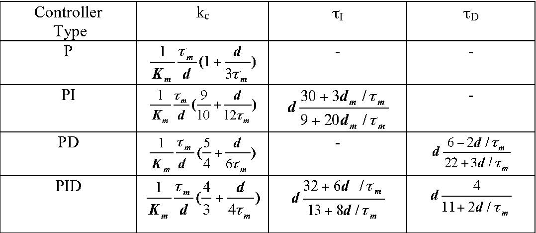
# 摘要
PID控制作为一种历史悠久的控制理论,一直广泛应用于工业自动化领域中。本文从基础理论讲起,详细分析了PID参数的理论分析与选择、调试实践技巧,并探讨了PID控制在多变量、模糊逻辑以及网络化和智能化方面的高级应用。通过案例分析,文章展示了PID控制在实际工业环境中的应用效果以及特殊环境下参数调整的策略。文章最后展望了PID控制技术的发展方
网络同步新境界:掌握G.7044标准中的ODU flex同步技术
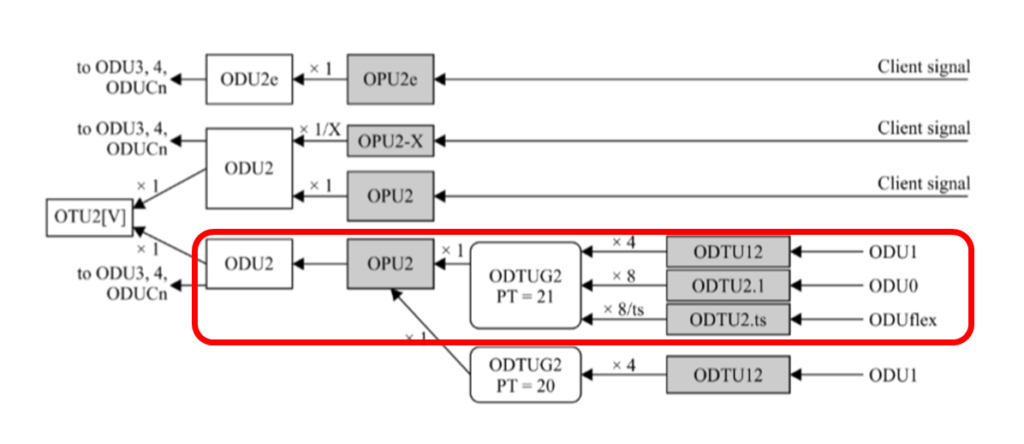
# 摘要
本文详细探讨了G.7044标准与ODU flex同步技术,首先介绍了该标准的技术原理,包括时钟同步的基础知识、G.7044标准框架及其起源与应用背景,以及ODU flex技术
字符串插入操作实战:insert函数的编写与优化
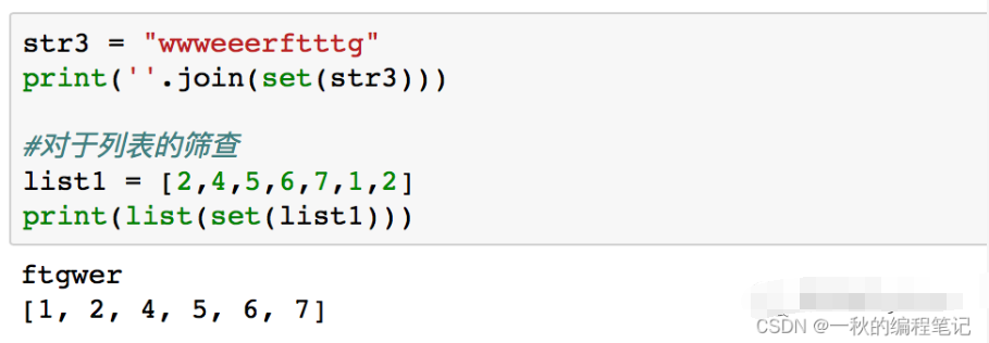
# 摘要
字符串插入操作是编程中常见且基础的任务,其效率直接影响程序的性能和可维护性。本文系统地探讨了字符串插入操作的理论基础、insert函数的编写原理、使用实践以及性能优化。首先,概述了insert函数的基本结构、关键算法和代码实现。接着,分析了在不同编程语言中insert函数的应用实践,并通过性能测试揭示了各种实现的差异。此外,本文还探讨了性能优化策略,包括内存使用和CPU效率提升,并介绍了高级数据结
环形菜单的兼容性处理

# 摘要
环形菜单作为一种用户界面元素,为软件和网页设计提供了新的交互体验。本文首先介绍了环形菜单的基本知识和设计理念,重点探讨了其通过HTML、CSS和JavaScript技术实现的方法和原理。然后,针对浏览器兼容性问题,提出了有效的解决方案,并讨论了如何通过测试和优化提升环形菜单的性能和用户体验。本
资源上传下载、课程学习等过程中有任何疑问或建议,欢迎提出宝贵意见哦~我们会及时处理!
点击此处反馈


专栏目录
最低0.47元/天 解锁专栏
买1年送3月
百万级
高质量VIP文章无限畅学
千万级
优质资源任意下载
C知道
免费提问 ( 生成式Al产品 )