【Mysteries of Residual Analysis】: Diagnostics and Solutions for Residuals in Linear Regression Models
发布时间: 2024-09-14 17:40:09 阅读量: 8 订阅数: 14 
# 1. Understanding Residual Analysis
In linear regression models, residual analysis plays a vital role. Understanding residual analysis is a key step in exploring the underlying patterns in data. Residuals are the differences between observed values and model predictions, and residual analysis aims to test whether a model fits the data well, identify outliers, and observe the variability of the data. By learning residual analysis, we can deeply understand the performance of linear regression models, laying a solid foundation for subsequent model optimization and problem-solving.
# 2.1 Linear Regression Principles Elucidated
Linear regression is a statistical method used to establish a linear relationship between independent variables and dependent variables. In practical applications, simple linear regression and multiple linear regression can be used to fit data, and the method of least squares can be used to solve for model parameters.
### 2.1.1 Simple Linear Regression
In simple linear regression, there is a linear relationship between one independent variable and one dependent variable. Specifically, given an independent variable $x$ and a dependent variable $y$, the linear regression model can be expressed as $y = ax + b$. Here, $a$ represents the slope, and $b$ represents the intercept.
```python
# Example of a simple linear regression model
from sklearn.linear_model import LinearRegression
# Create a linear regression model
model = LinearRegression()
# Fit the data
model.fit(X, y)
# Get the model parameters
slope = model.coef_
intercept = model.intercept_
```
The above code demonstrates how to perform simple linear regression fitting using the `scikit-learn` library in Python and obtain the model's slope and intercept parameters.
### 2.1.2 Multiple Linear Regression
Multiple linear regression considers the effects of multiple independent variables on the dependent variable. Suppose there are $p$ independent variables $x_1, x_2, ..., x_p$, the linear regression model can be represented as $y = a_1x_1 + a_2x_2 + ... + a_px_p + b$. Here, $a_1, a_2, ..., a_p$ are the coefficients for each independent variable.
```python
# Example of a multiple linear regression model
from sklearn.linear_model import LinearRegression
# Create a linear regression model
model = LinearRegression()
# Fit the data
model.fit(X, y)
# Get the model coefficients and intercept
coefficients = model.coef_
intercept = model.intercept_
```
The above code shows how to perform multiple linear regression fitting using the `scikit-learn` library in Python and obtain the model's coefficients and intercept parameters.
### 2.1.3 Least Squares Method
The least squares method is a common parameter estimation technique used in linear regression models, aiming to minimize the sum of squared residuals between actual observed values and model predictions. By minimizing the sum of squared residuals, the optimal model parameter estimates can be obtained.
```python
# Example of the least squares method
import numpy as np
# Construct data
X = np.array([[1, 1], [1, 2], [2, 2], [2, 3]])
y = np.dot(X, np.array([1, 2])) + 3
# Solve using the least squares method
coefficients, residuals, rank, s = np.linalg.lstsq(X, y, rcond=None)
# Get the model coefficients
coefficients
```
The above code demonstrates how to use the NumPy library to solve the least squares method and obtain the coefficients for a linear regression model.
## Summary
In this section, we delved into the fundamentals of linear regression models, including simple linear regression, multiple linear regression, and the least squares method. These contents lay the groundwork for understanding subsequent chapters on residual analysis.
# 3. Residual Diagnostic Methods
Residual diagnostics are a crucial part of linear regression models, as analyzing residuals can test whether the model meets the basic assumptions of linear regression, identify outliers, and evaluate the goodness of fit of the model. This chapter will introduce methods for residual diagnostics, including prediction tests for linear regression and the basic properties of residuals.
### 3.1 Prediction Tests for Linear Regression
In linear regression, we often need to validate the model's predictions to ensure the accuracy and reliability of the model. Residual analysis is a common method for prediction testing, and this section will introduce several common residual diagnostic plots and testing methods.
#### 3.1.1 Q-Q Plot
The Q-Q plot (Quantile-Quantile Plot) is a method used to test whether data conforms to a certain distribution. In linear regression, we can use the Q-Q plot to check whether residuals are approximately normally distributed. Here is an example of how to draw a Q-Q plot:
```python
# Draw a Q-Q plot
import scipy.stats as stats
import numpy as np
import matplotlib.pyplot as plt
residuals = model.resid # Assuming model is a linear regression model
stats.probplot(residuals, dist="norm", plot=plt)
plt.show()
```
By observing whether the points on the Q-Q plot approximately lie on a straight line, we can preliminarily judge whether the residuals conform to the normal distribution.
#### 3.1.2 Homoscedasticity Test
Another basic assumption of linear regression models is that the residual variance should be constant. To verify homoscedasticity, we can use a scatter plot of residuals to check if the residual variance is independent of the predicted values. Here is an example of how to perform a homoscedasticity test:
```python
# Draw a residual scatter plot
import matplotlib.pyplot as plt
plt.scatter(model.fittedvalues, model.resid)
plt.axhline(y=0, color='r', linestyle='--')
plt.xlabel('Fitted values')
plt.ylabel('Residuals')
plt.title('Residuals vs. Fitt
```

 百万级
高质量VIP文章无限畅学
百万级
高质量VIP文章无限畅学
 千万级
优质资源任意下载
千万级
优质资源任意下载
 C知道
免费提问 ( 生成式Al产品 )
C知道
免费提问 ( 生成式Al产品 )
0
0
相关推荐

专栏目录
最低0.47元/天 解锁专栏
送3个月
百万级
高质量VIP文章无限畅学
千万级
优质资源任意下载
C知道
免费提问 ( 生成式Al产品 )
最新推荐
Python在语音识别中的应用:构建能听懂人类的AI系统的终极指南

# 1. 语音识别与Python概述
在当今飞速发展的信息技术时代,语音识别技术的应用范围越来越广,它已经成为人工智能领域里一个重要的研究方向。Python作为一门广泛应用于数据科学和机器学习的编程语言,因其简洁的语法和强大的库支持,在语音识别系统开发中扮演了重要角色。本章将对语音识别的概念进行简要介绍,并探讨Python在语音识别中的应用和优势。
语音识别技术本质上是计算机系统通过算法将人类的语音信号转换
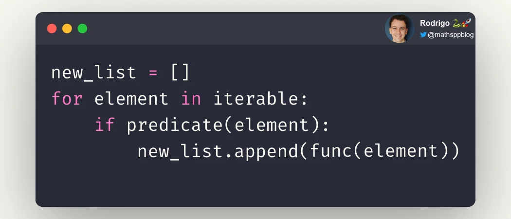
Python列表的函数式编程之旅:map和filter让代码更优雅
# 1. 函数式编程简介与Python列表基础
## 1.1 函数式编程概述
函数式编程(Functional Programming,FP)是一种编程范式,其主要思想是使用纯函数来构建软件。纯函数是指在相同的输入下总是返回相同输出的函数,并且没有引起任何可观察的副作用。与命令式编程(如C/C++和Java)不同,函数式编程
【Python调试技巧】:使用字符串进行有效的调试
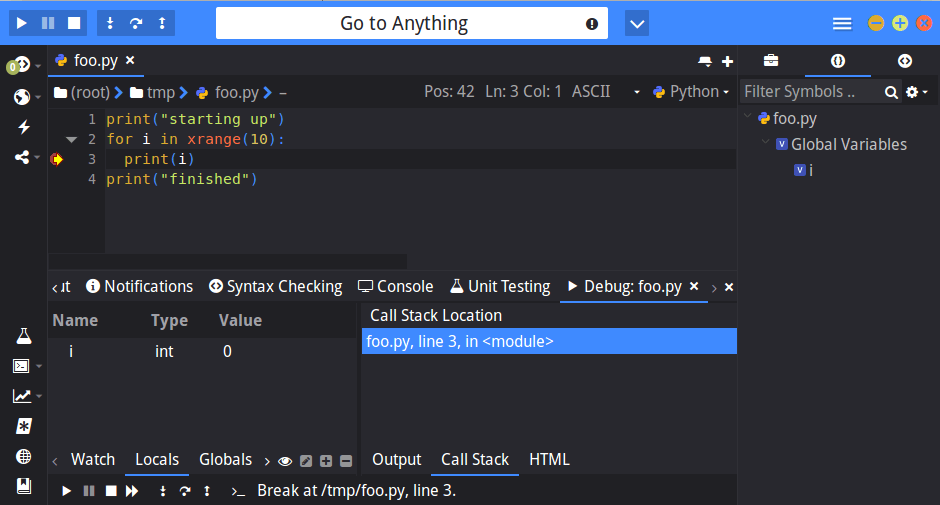
# 1. Python字符串与调试的关系
在开发过程中,Python字符串不仅是数据和信息展示的基本方式,还与代码调试紧密相关。调试通常需要从程序运行中提取有用信息,而字符串是这些信息的主要载体。良好的字符串使用习惯能够帮助开发者快速定位问题所在,优化日志记录,并在异常处理时提供清晰的反馈。这一章将探讨Python字符串与调试之间的关系,并展示如何有效地利用字符串进行代码调试。
# 2. P
Python测试驱动开发(TDD)实战指南:编写健壮代码的艺术
# 1. 测试驱动开发(TDD)简介
测试驱动开发(TDD)是一种软件开发实践,它指导开发人员首先编写失败的测试用例,然后编写代码使其通过,最后进行重构以提高代码质量。TDD的核心是反复进行非常短的开发周期,称为“红绿重构”循环。在这一过程中,"红"代表测试失败,"绿"代表测试通过,而"重构"则是在测试通过后,提升代码质量和设计的阶段。TDD能有效确保软件质量,促进设计的清晰度,以及提高开发效率。尽管它增加了开发初期的工作量,但长远来
Python内存管理与字符串转换:揭开工作原理的神秘面纱

# 1. Python内存管理机制概述
Python作为一种高级编程语言,其内存管理机制是支撑程序高效运行的关键技术之一。本章首先简要介绍
【持久化存储】:将内存中的Python字典保存到磁盘的技巧

# 1. 内存与磁盘存储的基本概念
在深入探讨如何使用Python进行数据持久化之前,我们必须先了解内存和磁盘存储的基本概念。计算机系统中的内存指的
【Python排序与异常处理】:优雅地处理排序过程中的各种异常情况
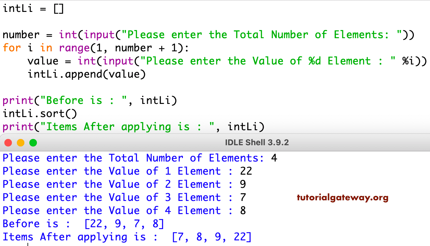
# 1. Python排序算法概述
排序算法是计算机科学中的基础概念之一,无论是在学习还是在实际工作中,都是不可或缺的技能。Python作为一门广泛使用的编程语言,内置了多种排序机制,这些机制在不同的应用场景中发挥着关键作用。本章将为读者提供一个Python排序算法的概览,包括Python内置排序函数的基本使用、排序算法的复杂度分析,以及高级排序技术的探
Python索引的局限性:当索引不再提高效率时的应对策略

# 1. Python索引的基础知识
在编程世界中,索引是一个至关重要的概念,特别是在处理数组、列表或任何可索引数据结构时。Python中的索引也不例外,它允许我们访问序列中的单个元素、切片、子序列以及其他数据项。理解索引的基础知识,对于编写高效的Python代码至关重要。
## 理解索引的概念
Python中的索引从0开始计数。这意味着列表中的第一个元素
Python并发控制:在多线程环境中避免竞态条件的策略

# 1. Python并发控制的理论基础
在现代软件开发中,处理并发任务已成为设计高效应用程序的关键因素。Python语言因其简洁易读的语法和强大的库支持,在并发编程领域也表现出色。本章节将为读者介绍并发控制的理论基础,为深入理解和应用Python中的并发工具打下坚实的基础。
## 1.1 并发与并行的概念区分
首先,理解并发和并行之间的区别至关重要。并发(Concurre
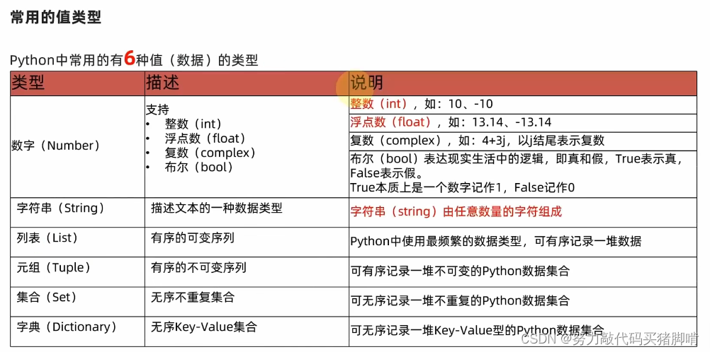
索引与数据结构选择:如何根据需求选择最佳的Python数据结构
# 1. Python数据结构概述
Python是一种广泛使用的高级编程语言,以其简洁的语法和强大的数据处理能力著称。在进行数据处理、算法设计和软件开发之前,了解Python的核心数据结构是非常必要的。本章将对Python中的数据结构进行一个概览式的介绍,包括基本数据类型、集合类型以及一些高级数据结构。读者通过本章的学习,能够掌握Python数据结构的基本概念,并为进一步深入学习奠
资源上传下载、课程学习等过程中有任何疑问或建议,欢迎提出宝贵意见哦~我们会及时处理!
点击此处反馈


专栏目录
最低0.47元/天 解锁专栏
送3个月
百万级
高质量VIP文章无限畅学
千万级
优质资源任意下载
C知道
免费提问 ( 生成式Al产品 )