揭秘无向图连通分量：探索图论内部结构的奥秘

# 1. 无向图的基本概念**

无向图是一种数据结构，由一组顶点和连接这些顶点的边组成。无向图中，边不具有方向性，即从顶点 A 到顶点 B 的边与从顶点 B 到顶点 A 的边是相同的。

无向图中的两个顶点被称为相连的，如果它们之间存在一条边。一个连通分量是一组相互连接的顶点，其中任何两个顶点之间都存在一条路径。一个无向图可以包含多个连通分量，每个连通分量是一个独立的子图。

# 2. 连通分量理论

### 2.1 连通分量的定义和性质

**定义：**

在无向图中，如果图中任意两点之间都存在一条路径，则称该图是连通的。连通图中的最大连通子图称为连通分量。

**性质：**

* 一个连通图只有一个连通分量。
* 一个连通分量中的所有点都是相互连通的。
* 一个无向图的连通分量个数等于图中边的个数减去点个数加 1。

### 2.2 连通分量的算法

**DFS 算法：**

深度优先搜索算法（DFS）可以用来求解无向图的连通分量。其基本思想是：

1. 从图中的任意一点开始，深度优先遍历图。
2. 遍历过程中，将遍历到的所有点标记为同一个连通分量。
3. 重复步骤 1 和 2，直到遍历完所有点。

**代码块：**

def dfs(graph, start):
    """
    深度优先搜索算法求连通分量

    Args:
        graph: 无向图，用邻接表表示
        start: 起始点
    """
    visited = set()  # 已访问的点集合
    component = []  # 当前连通分量

    def dfs_helper(node):
        if node in visited:
            return
        visited.add(node)
        component.append(node)
        for neighbor in graph[node]:
            dfs_helper(neighbor)

    dfs_helper(start)
    return component

**逻辑分析：**

* `dfs_helper` 函数是 DFS 算法的核心部分，它递归地遍历图，将遍历到的点标记为同一个连通分量。
* `visited` 集合用于记录已访问的点，避免重复访问。
* `component` 列表用于存储当前连通分量的所有点。

**BFS 算法：**

广度优先搜索算法（BFS）也可以用来求解无向图的连通分量。其基本思想是：

1. 从图中的任意一点开始，广度优先遍历图。
2. 遍历过程中，将遍历到的所有点标记为同一个连通分量。
3. 重复步骤 1 和 2，直到遍历完所有点。

**代码块：**

def bfs(graph, start):
    """
    广度优先搜索算法求连通分量

    Args:
        graph: 无向图，用邻接表表示
        start: 起始点
    """
    visited = set()  # 已访问的点集合
    component = []  # 当前连通分量
    queue = [start]  # 队列，用于存储待访问的点

    while queue:
        node = queue.pop(0)
        if node in visited:
            continue
        visited.add(node)
        component.append(node)
        for neighbor in graph[node]:
            if neighbor not in visited:
                queue.append(neighbor)

    return component

**逻辑分析：**

* `bfs` 函数是 BFS 算法的核心部分，它使用队列来广度优先遍历图，将遍历到的点标记为同一个连通分量。
* `visited` 集合用于记录已访问的点，避免重复访问。
* `component` 列表用于存储当前连通分量的所有点。

**并查集算法：**

并查集算法是一种高效的数据结构，可以用来求解无向图的连通分量。其基本思想是：

1. 初始化一个并查集，每个点都属于自己的连通分量。
2. 对于图中的每条边，将边的两个端点所在的连通分量合并。
3. 重复步骤 2，直到所有边都处理完。

**代码块：**

class UnionFind:
    def __init__(self, n):
        self.parent = list(range(n))
        self.size = [1] * n

    def find(self, x):
        if self.parent[x] != x:
            self.parent[x] = self.find(self.parent[x])
        return self.parent[x]

    def union(self, x, y):
        root_x = self.find(x)
        root_y = self.find(y)
        if root_x != root_y:
            if self.size[root_x] > self.size[root_y]:
                self.parent[root_y] = root_x
                self.size[root_x] += self.size[root_y]
            else:
                self.parent[root_x] = root_y
                self.size[root_y] += self.size[root_x]

def find_connected_components(graph):
    """
    并查集算法求连通分量

    Args:
        graph: 无向图，用邻接表表示
    """
    n = len(graph)
    uf = UnionFind(n)
    for edge in graph:
        x, y = edge
        uf.union(x, y)
    components = {}
    for i in range(n):
        root = uf.find(i)
        if root not in components:
            components[root] = []
        components[root].append(i)
    return list(components.values())

**逻辑分析：**

* `UnionFind` 类实现了并查集数据结构，其中 `parent` 数组记录每个点的父节点，`size` 数组记录每个连通分量的规模。
* `find` 函数用于查找一个点的根节点。
* `union` 函数用于合并两个连通分量。
* `find_connected_components` 函数使用并查集算法求解无向图的连通分量，并返回一个列表，其中每个元素是一个连通分量。

**表格：**

| 算法 | 时间复杂度 | 空间复杂度 |
|---|---|---|
| DFS | O(V + E) | O(V) |
| BFS | O(V + E) | O(V) |
| 并查集 | O(E log V) | O(V) |

**注：**

* V 为图中的点个数
* E 为图中的边个数

# 3.1 深度优先搜索算法

深度优先搜索（DFS）算法是一种遍历无向图的递归算法，它通过深度优先的方式探索图中的每个节点及其邻接节点。DFS 算法从图中的一个起始节点开始，并沿着一条路径一直向下探索，直到达到一个叶子节点（没有未访问的邻接节点）。然后，算法回溯到最近一个未完全探索的节点，并继续沿着另一条路径探索，直到所有节点都被访问。

**算法步骤：**

1. 从图中的一个起始节点开始，将其标记为已访问。
2. 对于当前节点的每个未访问的邻接节点：
- 递归调用 DFS 算法，从该邻接节点开始。
3. 当当前节点的所有邻接节点都已访问后，回溯到最近一个未完全探索的节点。
4. 重复步骤 2 和 3，直到所有节点都被访问。

**代码实现：**

def dfs(graph, start_node):
    """
    深度优先搜索算法

    参数：
        graph: 无向图，以邻接表的形式表示
        start_node: 起始节点
    """
    visited = set()  # 已访问节点集合

    def dfs_recursive(node):
        if node in visited:
            return
        visited.add(node)
        for neighbor in graph[node]:
            dfs_recursive(neighbor)

    dfs_recursive(start_node)

**逻辑分析：**

* `visited` 集合用于跟踪已访问的节点。
* `dfs_recursive` 函数是 DFS 算法的递归实现。
* 如果当前节点已访问，则直接返回。
* 否则，将当前节点标记为已访问，并遍历其所有未访问的邻接节点。
* 对于每个邻接节点，递归调用 `dfs_recursive` 函数，继续探索该节点及其邻接节点。

**参数说明：**

* `graph`: 无向图，以邻接表的形式表示，其中键为节点，值为该节点的邻接节点列表。
* `start_node`: DFS 算法的起始节点。

### 3.2 广度优先搜索算法

广度优先搜索（BFS）算法也是一种遍历无向图的算法，但它采用广度优先的方式探索图中的节点。BFS 算法从图中的一个起始节点开始，并首先访问该节点的所有邻接节点。然后，算法访问这些邻接节点的所有未访问的邻接节点，依此类推，直到所有节点都被访问。

**算法步骤：**

1. 从图中的一个起始节点开始，将其加入一个队列中。
2. 只要队列不为空：
- 从队列中取出一个节点，并将其标记为已访问。
- 对于当前节点的每个未访问的邻接节点：
- 将该邻接节点加入队列中。
3. 重复步骤 2，直到所有节点都被访问。

**代码实现：**

def bfs(graph, start_node):
    """
    广度优先搜索算法

    参数：
        graph: 无向图，以邻接表的形式表示
        start_node: 起始节点
    """
    visited = set()  # 已访问节点集合
    queue = [start_node]  # 队列

    while queue:
        node = queue.pop(0)  # 从队列中取出一个节点
        if node in visited:
            continue
        visited.add(node)
        for neighbor in graph[node]:
            if neighbor not in visited:
                queue.append(neighbor)

**逻辑分析：**

* `visited` 集合用于跟踪已访问的节点。
* `queue` 队列用于存储待访问的节点。
* 算法从队列中取出一个节点，并将其标记为已访问。
* 然后，遍历该节点的所有未访问的邻接节点，并将其加入队列中。
* 算法重复此过程，直到队列为空，即所有节点都被访问。

**参数说明：**

* `graph`: 无向图，以邻接表的形式表示，其中键为节点，值为该节点的邻接节点列表。
* `start_node`: BFS 算法的起始节点。

# 4. 连通分量应用

### 4.1 图的连通性判断

连通分量可以用来判断一个无向图是否连通。如果一个图的所有顶点都属于同一个连通分量，则该图是连通的；否则，该图是不连通的。

**算法步骤：**

1. 遍历图中的所有顶点，并对每个顶点执行深度优先搜索或广度优先搜索算法。
2. 对于每个顶点，记录其访问过的所有顶点。
3. 如果所有顶点都被访问过，则该图是连通的；否则，该图是不连通的。

**代码示例（Python）：**

def is_connected(graph):
    """判断一个无向图是否连通。

    参数：
        graph: 一个无向图，表示为邻接表。

    返回：
        如果图连通，返回 True；否则，返回 False。
    """

    # 初始化访问过的顶点集合
    visited = set()

    # 遍历图中的所有顶点
    for vertex in graph:
        # 如果该顶点未被访问过，则执行深度优先搜索
        if vertex not in visited:
            dfs(graph, vertex, visited)

    # 如果所有顶点都被访问过，则图是连通的
    return len(visited) == len(graph)


def dfs(graph, vertex, visited):
    """深度优先搜索算法。

    参数：
        graph: 一个无向图，表示为邻接表。
        vertex: 当前访问的顶点。
        visited: 已访问的顶点集合。
    """

    # 将当前顶点标记为已访问
    visited.add(vertex)

    # 遍历当前顶点的所有邻接顶点
    for neighbor in graph[vertex]:
        # 如果邻接顶点未被访问过，则递归调用深度优先搜索
        if neighbor not in visited:
            dfs(graph, neighbor, visited)

### 4.2 图的割点和桥的识别

**割点：**一个顶点，如果将其从图中移除，会使图的连通分量数增加。

**桥：**一条边，如果将其从图中移除，会使图的连通分量数增加。

**算法步骤：**

1. 对图执行深度优先搜索算法。
2. 记录每个顶点的发现时间和最低时间。
3. 对于每个顶点，如果其最低时间大于其发现时间，则该顶点是割点。
4. 对于每条边，如果其两端顶点的最低时间不同，则该边是桥。

**代码示例（Python）：**

def find_cut_vertices_and_bridges(graph):
    """找到图中的割点和桥。

    参数：
        graph: 一个无向图，表示为邻接表。

    返回：
        一个元组，包含割点列表和桥列表。
    """

    # 初始化发现时间和最低时间
    discovery_time = {}
    low_time = {}
    parent = {}
    cut_vertices = set()
    bridges = set()

    # 初始化时间戳
    time = 0

    # 对图执行深度优先搜索
    for vertex in graph:
        if vertex not in discovery_time:
            dfs(graph, vertex, parent, discovery_time, low_time, cut_vertices, bridges, time)

    return cut_vertices, bridges


def dfs(graph, vertex, parent, discovery_time, low_time, cut_vertices, bridges, time):
    """深度优先搜索算法。

    参数：
        graph: 一个无向图，表示为邻接表。
        vertex: 当前访问的顶点。
        parent: 当前顶点的父顶点。
        discovery_time: 顶点的发现时间。
        low_time: 顶点的最低时间。
        cut_vertices: 割点列表。
        bridges: 桥列表。
        time: 时间戳。
    """

    # 将当前顶点的发现时间和最低时间设置为当前时间戳
    discovery_time[vertex] = time
    low_time[vertex] = time

    # 遍历当前顶点的所有邻接顶点
    for neighbor in graph[vertex]:
        # 如果邻接顶点未被访问过
        if neighbor not in discovery_time:
            # 将当前顶点设置为邻接顶点的父顶点
            parent[neighbor] = vertex

            # 递归调用深度优先搜索
            dfs(graph, neighbor, parent, discovery_time, low_time, cut_vertices, bridges, time + 1)

            # 更新当前顶点的最低时间
            low_time[vertex] = min(low_time[vertex], low_time[neighbor])

            # 如果当前顶点的最低时间大于其发现时间，则当前顶点是割点
            if low_time[neighbor] >= discovery_time[vertex]:
                cut_vertices.add(vertex)

        # 如果邻接顶点已被访问过，并且不是当前顶点的父顶点
        elif neighbor != parent[vertex]:
            # 更新当前顶点的最低时间
            low_time[vertex] = min(low_time[vertex], discovery_time[neighbor])

            # 如果当前顶点的最低时间大于其发现时间，并且邻接顶点的发现时间小于当前顶点的发现时间
            if low_time[vertex] > discovery_time[vertex] and discovery_time[neighbor] < discovery_time[vertex]:
                # 当前顶点和邻接顶点之间的边是桥
                bridges.add((vertex, neighbor))

### 4.3 图的最小生成树

**最小生成树：**一个图的生成树，其权重和最小。

**算法步骤：**

1. 对图执行普里姆算法或克鲁斯卡尔算法。
2. 算法将生成一个最小生成树。

**代码示例（Python）：**

**普里姆算法：**

def prim_mst(graph, weights):
    """使用普里姆算法找到图的最小生成树。

    参数：
        graph: 一个无向图，表示为邻接表。
        weights: 图中边的权重，表示为一个字典，键为边，值为权重。

    返回：
        一个最小生成树，表示为一个字典，键为边，值为权重。
    """

    # 初始化最小生成树
    mst = {}

    # 初始化已访问的顶点集合
    visited = set()

    # 初始化当前顶点
    current_vertex = next(iter(graph))

    # 遍历图中的所有顶点
    while current_vertex is not None:
        # 将当前顶点添加到已访问的顶点集合中
        visited.add(current_vertex)

        # 遍历当前顶点的所有邻接顶点
        for neighbor in graph[current_vertex]:
            # 如果邻接顶点未被访问过，并且当前顶点和邻接顶点之间的边权重小于最小生成树中边的权重
            if neighbor not in visited and (current_vertex, neighbor) not in mst and (neighbor, current_vertex) not in mst:
                # 将当前顶点和邻接顶点之间的边添加到最小生成树中
                mst[(current_vertex, neighbor)] = weights[(current_vertex, neighbor)]

        # 找到已访问的顶点集合中权重最小的边
        min_weight = float('inf')
        min_edge = None
        for vertex in visited:
            for neighbor in graph[vertex]:
                if neighbor not in visited and (vertex, neighbor) not in mst and (neighbor, vertex) not in mst:
                    if weights[(vertex, neighbor)] < min_weight:
                        min_weight = weights[(vertex, neighbor)]
                        min_edge = (vertex, neighbor)

        # 将权重最小的边添加到最小生成树中
        if min_edge is not None:
            mst[min_edge] = min_weight

        # 更新当前顶点
        current_vertex = min_edge[1] if min_edge is not None else None

    return mst

**克鲁斯卡尔算法：**

def kruskal_mst(graph, weights):
    """使用克鲁斯卡尔算法找到图的最小生成树。

    参数：
        graph: 一个无向图，表示为邻接表。
        weights: 图中边的权重，表示为一个字典，键为边，值为权重。

    返回：
        一个最小生成树，表示为一个字典，键为边，值为权重。
    """

    # 初始化并查集
    disjoint_set = DisjointSet()

    # 将图中的所有顶点添加到并查集中
    for vertex in graph:
        disjoint_set.make_set(vertex)

    # 初始化最小生成树
    mst = {}

    # 遍历图中的所有边
    for edge

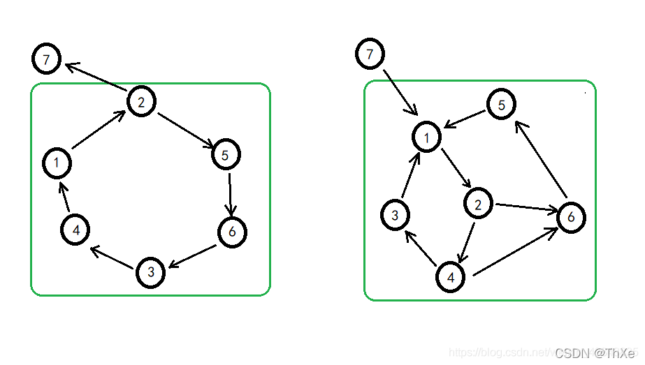
# 5.1 强连通分量

在无向图中，连通分量是指图中任意两点之间都存在路径。而在有向图中，我们引入了强连通分量的概念。

**定义：**

强连通分量是一个有向图中的子图，其中图中的任意两个顶点之间都存在一条有向路径。

**性质：**

* 一个强连通分量中的所有顶点都互相可达。
* 一个有向图可以被分解为多个强连通分量，这些强连通分量互不相交。
* 一个强连通分量中的所有顶点都有相同的入度和出度。

**算法：**

求解有向图的强连通分量可以使用 Kosaraju 算法：

1. **第一遍 DFS：**从任意顶点出发，对整个图进行深度优先搜索（DFS），记录每个顶点的完成时间。
2. **逆转有向图：**将有向图的所有边反转，得到逆向图。
3. **第二遍 DFS：**从完成时间最大的顶点出发，对逆向图进行深度优先搜索，记录每个顶点所在的强连通分量。

**代码：**

def kosaraju(graph):
"""
求解有向图的强连通分量

参数：
graph: 有向图，邻接表表示

返回：
强连通分量列表
"""

# 第一遍 DFS
visited = set()
finishing_time = {}
stack = []

def dfs1(node):
if node in visited:
return

visited.add(node)
for neighbor in graph[node]:
dfs1(neighbor)

stack.append(node)

for node in graph:
dfs1(node)

# 逆转有向图
reversed_graph = {node: [] for node in graph}
for node in graph:
for neighbor in graph[node]:
reversed_graph[neighbor].append(node)

# 第二遍 DFS
visited = set()
scc = []

def dfs2(node):
if node in visited:
return

visited.add(node)
scc.append(node)

for neighbor in reversed_graph[node]:
dfs2(neighbor)

while stack:
node = stack.pop()
if node not in visited:
dfs2(node)
scc.append([])

return scc