【fmincon Optimization Algorithm: Mastering the Principles, Parameters, and Applications in 10 Steps】
发布时间: 2024-09-14 11:29:18 阅读量: 49 订阅数: 27 
# Step-by-Step Mastery of the fmincon Optimization Algorithm: Principles, Parameters, and Applications
## 1. Overview of the fmincon Optimization Algorithm
The fmincon algorithm is a nonlinear constrained optimization technique used to solve optimization problems with constraints. It is widely applied in various fields such as engineering design, financial investment, and machine learning. Based on the Sequential Quadratic Programming (SQP) method, fmincon iteratively approaches the optimal solution.
## 2. Principles of the fmincon Optimization Algorithm
### 2.1 Constrained Optimization Problems
Constrained optimization problems aim to find the optimal value of an objective function while satisfying certain constraints. These constraints can be equality constraints or inequality constraints.
**Equality Constraints:** Represented as `h(x) = 0`, where `h(x)` is a vector function.
**Inequality Constraints:** Represented as `g(x) <= 0`, where `g(x)` is a vector function.
### 2.2 Mathematical Foundations of the fmincon Algorithm
The fmincon algorithm is based on the **Feasible Domain Method**, which searches for the optimal solution through iterative exploration of the feasible domain (the region that satisfies all constraints). The mathematical underpinnings of the algorithm include:
- **Lagrange Multiplier Method:** Transforms constraints into a Lagrangian function, and the optimal feasible solution is found by seeking the extremum of the Lagrangian function.
- **Feasible Direction Method:** At the current feasible point, finds a feasible direction along which moving can reduce the objective function value.
- **Trust-Region Method:** Establishes a trust region near the current point, approximates the objective function and constraints within the trust region, and solves for the optimal solution of the approximated problem.
### 2.3 Solving Process and Algorithm Flow
The solving process of the fmincon algorithm mainly includes the following steps:
1. **Initialization:** Set the initial point, objective function, constraints, and optimization options.
2. **Feasibility Check:** Check if the initial point satisfies the constraints.
3. **Feasible Direction Search:** Find a feasible direction along which moving can reduce the objective function value.
4. **Step Size Determination:** Determine the step size along the feasible direction to satisfy the constraints and optimization goals.
5. **Update the Feasible Point:** Move along the feasible direction with the step size and update the current feasible point.
6. **Feasibility Recheck:** Check if the updated feasible point satisfies the constraints.
7. **Convergence Judgment:** Check if convergence conditions are met; if yes, stop iteration; otherwise, return to step 3.
**Algorithm Flowchart:**
```mermaid
graph LR
subgraph fmincon Algorithm Flow
init[Initialization] --> check[Feasibility Check]
check --> search[Feasible Direction Search]
search --> step[Step Size Determination]
step --> update[Update Feasible Point]
update --> check
check --> converge[Convergence Judgment]
converge --> end[End]
end
```
### Code Example
```python
import numpy as np
from scipy.optimize import fmincon
def objective_function(x):
return x[0]**2 + x[1]**2
def constraint_function(x):
return np.array([x[0] + x[1] - 1, x[0] - x[1]])
# Solving the constrained optimization problem
x0 = np.array([0, 0]) # Initial point
bounds = [(None, None), (None, None)] # Variable bounds
cons = ({'type': 'ineq', 'fun': constraint_function}) # Constraints
# Solve
result = fmincon(objective_function, x0, bounds=bounds, constraints=cons)
# Output the results
print('Optimal solution:', result.x)
print('Optimal value:', result.fun)
```
**Code Logic Analysis:**
* `objective_function` defines the objective function.
* `constraint_function` defines the constraint conditions.
* The `fmincon` function solves the constrained optimization problem and returns the optimal solution and its value.
* `bounds` specifies the bounds of variables, where `None` indicates no bound.
* `cons` specifies the constraint conditions, where `'type'` indicates the type of constraint (equality or inequality), and `'fun'` indicates the constraint function.
## 3.1 Optimizing the Objective Function
**Definition:**
The objective function is what the fmincon algorithm aims to minimize. It represents the target to be optimized and can be any differentiable scalar function.
**Parameters:**
* `fun`: A handle to the objective function that takes a vector input (design variables) and returns a scalar output (objective value).
**Code Example:**
```matlab
% Defining the objective function
fun = @(x) x(1)^2 + x(2)^2;
% Setting optimization options
options = optimoptions('fmincon');
% Solving the optimization problem
[x, fval] = fmincon(fun, [0, 0], [], [], [], [], [], [], [], options);
```
**Logic Analysis:**
* The `fun` function defines the objective function, calculating the sum of squares of two design variables.
* The `options` variable sets optimization options, including algorithm parameters and termination criteria.
* The `fmincon` function minimizes the objective function using the specified optimization options.
* The `x` variable stores the optimized design variables, and `fval` variable stores the minimized objective value.
### 3.2 Constraint Conditions
**Definition:**
Constraint conditions limit the range of design variables to ensure that the solution meets specific requirements or restrictions. The fmincon algorithm supports various types of constraints, including:
***Linear Constraints:** `Ax <= b`
***Nonlinear Constraints:** `c(x) <= 0` or `c(x) = 0`
**Parameters:**
* `A` and `b`: The coefficient matrix and right-hand side vector for linear constraints.
* `c`: The function handle for nonlinear constraints.
**Code Example:**
```matlab
% Defining linear constraints
A = [1, -1; -1, 1];
b = [1; 1];
% Defining nonlinear constraints
c = @(x) x(1)^2 + x(2)^2 - 1;
% Setting optimization options
options = optimoptions('fmincon');
% Solving the optimization problem
[x, fval] = fmincon(fun, [0, 0], A, b, [], [], [], [], c, options);
```
**Logic Analysis:**
* `A` and `b` define the linear constraints, requiring the sum and difference of the design variables to be less than or equal to 1.
* The `c` function defines the nonlinear constraint, requiring the sum of squares of the design variables to be less than or equal to 1.
* The `fmincon` function minimizes the objective function using the specified constraint conditions.
### 3.3 Optimization Options and Parameter Settings
**Definition:**
Optimization options and parameter settings allow users to customize the behavior of the fmincon algorithm, including:
***Algorithm Selection:** The `Algorithm` parameter specifies the optimization algorithm used, such as the interior-point or active-set methods.
***Termination Criteria:** The `TolFun` and `TolX` parameters set the tolerances for the objective function value and design variable changes to determine when the algorithm stops.
***Display Options:** The `Display` parameter controls the display output of the algorithm, such as iteration information and optimization progress.
**Parameters:**
* `Algorithm`: The choice of optimization algorithm.
* `TolFun`: Tolerance for objective function value.
* `TolX`: Tolerance for design variable changes.
* `Display`: Display options.
**Code Example:**
```matlab
% Setting optimization options
options = optimoptions('fmincon');
options.Algorithm = 'interior-point';
options.TolFun = 1e-6;
options.TolX = 1e-6;
options.Display = 'iter';
% Solving the optimization problem
[x, fval] = fmincon(fun, [0, 0], [], [], [], [], [], [], [], options);
```
**Logic Analysis:**
* The `options` variable sets optimization options, including the interior-point algorithm, strict tolerances, and detailed display output.
* The `fmincon` function minimizes the objective function using the specified optimization options.
## 4. Practical Applications of the fmincon Optimization Algorithm
### 4.1 Example of Engineering Design Optimization
#### Problem Description
An automobile manufacturer needs to design a new car chassis to maximize fuel efficiency and stability. Design variables include the chassis's length, width, and height, as well as the stiffness and damping coefficients of the suspension system.
#### fmincon Solving Process
Using the fmincon optimization algorithm, the fuel efficiency and stability are taken as the objective functions, while the chassis dimensions and suspension parameters are taken as design variables. Constraints include the minimum and maximum sizes of the chassis and the range of stiffness and damping coefficients for the suspension system.
```python
import numpy as np
from scipy.optimize import fmincon
# Defining the optimization objective function
def objective_function(x):
# x[0]: length, x[1]: width, x[2]: height, x[3]: stiffness, x[4]: damping coefficient
fuel_efficiency = ... # Calculate fuel efficiency
stability = ... # Calculate stability
return -fuel_efficiency - stability # The negative sign indicates maximization
# Defining the constraint conditions
def constraints(x):
# Length constraints
length_min = ...
length_max = ...
# Width constraints
width_min = ...
width_max = ...
# Height constraints
height_min = ...
height_max = ...
# Stiffness constraints
stiffness_min = ...
stiffness_max = ...
# Damping coefficient constraints
damping_min = ...
damping_max = ...
return [
length_min - x[0],
x[0] - length_max,
width_min - x[1],
x[1] - width_max,
height_min - x[2],
x[2] - height_max,
stiffness_min - x[3],
x[3] - stiffness_max,
damping_min - x[4],
x[4] - damping_max,
]
# Setting optimization options
options = {'maxiter': 1000}
# Solving the optimization problem
x_opt, fval, _, _, _ = fmincon(objective_function, x0, constraints, options=options)
```
#### Result Analysis
The fmincon algorithm found the optimal design parameters, maximizing fuel efficiency and stability. By analyzing the optimization results, engineers can determine the optimal dimensions for the chassis and the best settings for the suspension system, thus designing an excellent car chassis.
### 4.2 Example of Financial Portfolio Optimization
#### Problem Description
An investor wishes to construct a portfolio to maximize returns while controlling risks. The portfolio consists of stocks, bonds, and cash, and each asset class's weight needs to be optimized.
#### fmincon Solving Process
Using the fmincon optimization algorithm, returns are taken as the optimization objective function, while the portfolio weights are taken as design variables. Constraints include the sum of weights being equal to 1 and the risk limits for each asset class.
```python
import numpy as np
from scipy.optimize import fmincon
# Defining the optimization objective function
def objective_function(x):
# x[0]: stock weight, x[1]: bond weight, x[2]: cash weight
return ... # Calculate returns
# Defining the constraint conditions
def constraints(x):
# Sum of weights equals 1
weight_sum = ...
# Stock risk constraint
stock_risk = ...
stock_risk_max = ...
# Bond risk constraint
bond_risk = ...
bond_risk_max = ...
return [
weight_sum - 1,
stock_risk - stock_risk_max,
bond_risk - bond_risk_max,
]
# Setting optimization options
options = {'maxiter': 1000}
# Solving the optimization problem
x_opt, fval, _, _, _ = fmincon(objective_function, x0, constraints, options=options)
```
#### Result Analysis
The fmincon algorithm found the optimal portfolio weights, achieving maximized returns and controlled risks. By analyzing the optimization results, investors can determine the best allocation for stocks, bonds, and cash, thus constructing a portfolio with an excellent risk-return ratio.
### 4.3 Example of Machine Learning Model Tuning
#### Problem Description
The performance of a machine learning model depends on its hyperparameter settings. These need to be optimized to improve the model's accuracy and generalization ability.
#### fmincon Solving Process
Using the fmincon optimization algorithm, model evaluation metrics (such as accuracy or cross-validation score) are taken as the optimization objective function, while hyperparameters are taken as design variables. Constraints can include the range of hyperparameter values.
```python
import numpy as np
from scipy.optimize import fmincon
# Defining the optimization objective function
def objective_function(x):
# x[0]: hyperparameter 1, x[1]: hyperparameter 2, ...
model = ... # Create machine learning model
model.set_params(x) # Set hyperparameters
score = ... # Calculate model evaluation metric
return -score # The negative sign indicates maximization
# Defining the constraint conditions
def constraints(x):
# Hyperparameter 1 constraint
param1_min = ...
param1_max = ...
# Hyperparameter 2 constraint
param2_min = ...
param2_max = ...
return [
param1_min - x[0],
x[0] - param1_max,
param2_min - x[1],
x[1] - param2_max,
]
# Setting optimization options
options = {'maxiter': 1000}
# Solving the optimization problem
x_opt, fval, _, _, _ = fmincon(objective_function, x0, constraints, options=options)
```
#### Result Analysis
The fmincon algorithm found the optimal hyperparameter settings, enhancing the performance of the machine learning model. By analyzing the optimization results, the best hyperparameter combination for the model can be determined, thus constructing a machine learning model with higher accuracy and generalization ability.
## 5.1 Handling Complex Constraint Conditions
The fmincon algorithm can handle various constraint conditions, including linear constraints, nonlinear constraints, and integer constraints. For complex constraints, the following techniques can be used:
- **Decomposing Complex Constraints:** Break down complex constraints into multiple sub-constraints and handle each one separately.
- **Using Penalty Function Method:** Convert constraint conditions into penalty functions and add penalty function terms to the objective function. The algorithm will automatically consider the constraints.
- **Using Projection Method:** Project the feasible solution onto a subspace that satisfies the constraint conditions and then optimize within the subspace.
```python
import numpy as np
from scipy.optimize import fmin_slsqp
def objective_function(x):
return x[0]**2 + x[1]**2
def constraint_function(x):
return np.array([x[0] + x[1] - 1,
x[0] - x[1]])
# Using the penalty function method
penalty_factor = 100
def penalized_objective_function(x):
return objective_function(x) + penalty_factor * np.sum(np.maximum(0, constraint_function(x))**2)
# Solve
x0 = np.array([0.5, 0.5])
result = fmin_slsqp(penalized_objective_function, x0, fprime=None, fconstr=constraint_function)
print(result)
```
## 5.2 Solving Multi-Objective Optimization Problems
The fmincon algorithm can be extended to solve multi-objective optimization problems. For multi-objective optimization problems, multiple objective functions need to be defined, and weighting factors are used to perform a weighted sum.
```python
import numpy as np
from scipy.optimize import fmin_cobyla
def objective_function(x):
return [x[0]**2, x[1]**2]
def constraint_function(x):
return np.array([x[0] + x[1] - 1])
# Using the weighted sum method
weights = np.array([0.5, 0.5])
def weighted_objective_function(x):
return np.dot(weights, objective_function(x))
# Solve
x0 = np.array([0.5, 0.5])
result = fmin_cobyla(weighted_objective_function, x0, fprime=None, fconstr=constraint_function)
print(result)
```
## 5.3 Tips for Optimizing Algorithm Performance
To enhance the performance of the fmincon algorithm, the following tips can be used:
- **Choose the appropriate solver:** Select a suitable solver based on the type and scale of the optimization problem.
- **Set reasonable initial values:** Providing reasonable initial values can speed up the convergence rate.
- **Use gradient information:** If the objective function and constraints have gradient information, using this can improve algorithm efficiency.
- **Parallelize computations:** For large-scale optimization problems, parallelizing computations can increase the speed of the algorithm.

 百万级
高质量VIP文章无限畅学
百万级
高质量VIP文章无限畅学
 千万级
优质资源任意下载
千万级
优质资源任意下载
 C知道
免费提问 ( 生成式Al产品 )
C知道
免费提问 ( 生成式Al产品 )
0
0
相关推荐

专栏目录
最低0.47元/天 解锁专栏
买1年送3月
百万级
高质量VIP文章无限畅学
千万级
优质资源任意下载
C知道
免费提问 ( 生成式Al产品 )
最新推荐
Android应用中的MAX30100集成完全手册:一步步带你上手
# 摘要
本文综合介绍了MAX30100传感器的搭建和应用,涵盖了从基础硬件环境的搭建到高级应用和性能优化的全过程。首先概述了MAX30100的工作原理及其主要特性,然后详细阐述了如何集成到Arduino或Raspberry Pi等开发板,并搭建相应的硬件环境。文章进一步介绍了软件环境的配置,包括Arduino IDE的安装、依赖库的集成和MAX30100库的使用。接着,通过编程实践展示了MAX30100的基本操作和高级功能的开发,包括心率和血氧饱和度测量以及与Android设备的数据传输。最后,文章探讨了MAX30100在Android应用中的界面设计、功能拓展和性能优化,并通过实际案例分析
【AI高手】:掌握这些技巧,A*算法解决8数码问题游刃有余
# 摘要
A*算法是计算机科学中广泛使用的一种启发式搜索算法,尤其在路径查找和问题求解领域表现出色。本文首先概述了A*算法的基本概念,随后深入探讨了其理论基础,包括搜索算法的分类和评价指标,启发式搜索的原理以及评估函数的设计。通过结合著名的8数码问题,文章详细介绍了A*算法的实际操作流程、编码前的准备、实现步骤以及优化策略。在应用实例部分,文章通过具体问题的实例化和算法的实现细节,提供了深入的案例分析和问题解决方法。最后,本文展望
【硬件软件接口艺术】:掌握提升系统协同效率的关键策略
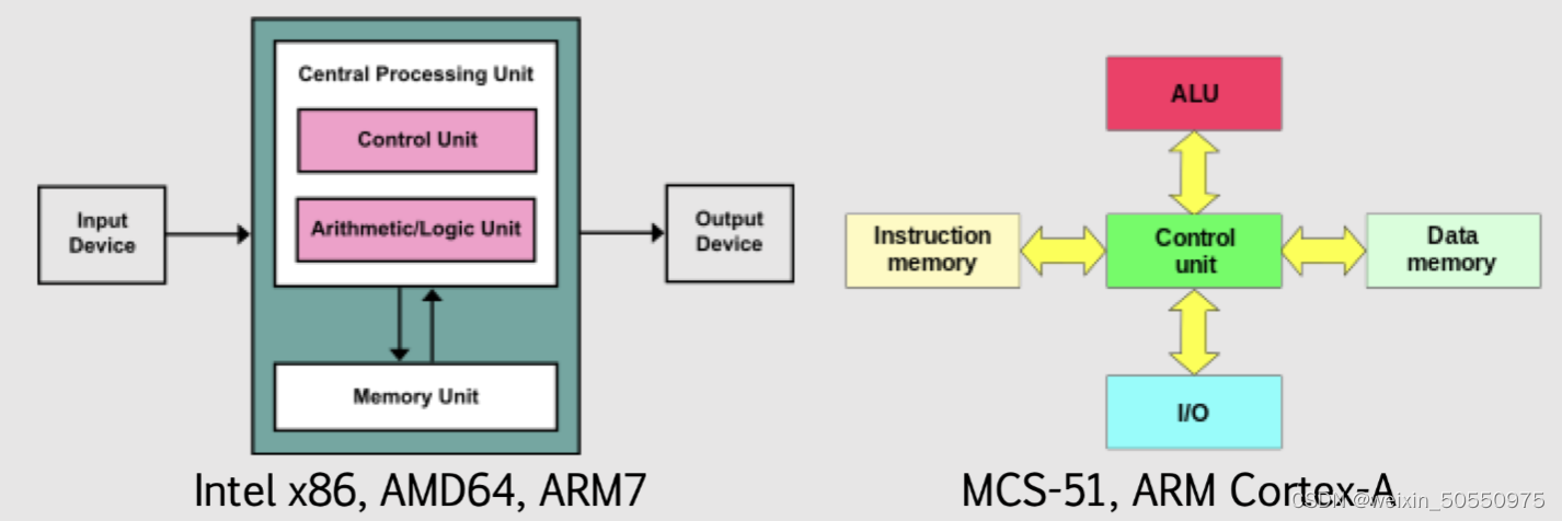
# 摘要
硬件与软件接口是现代计算系统的核心,它决定了系统各组件间的通信效率和协同工作能力。本文首先概述了硬件与软件接口的基本概念和通信机制,深入探讨了硬件通信接口标准的发展和主流技术的对比。接着,文章分析了软件接口的抽象层次,包括系统调用、API以及驱动程序的作用。此外,本文还详细介绍了同步与异步处理机制的原理和实践。在探讨提升系统协同效率的关键技术方面,文中阐述了缓存机制优化、多线程与并行处理,以及
PFC 5.0二次开发宝典:API接口使用与自定义扩展
# 摘要
本文深入探讨了PFC 5.0的技术细节、自定义扩展的指南以及二次开发的实践技巧。首先,概述了PFC 5.0的基础知识和标准API接口,接着详细分析了AP
【台达VFD-B变频器与PLC通信集成】:构建高效自动化系统的不二法门

# 摘要
本文综合介绍了台达VFD-B变频器与PLC通信的关键技术,涵盖了通信协议基础、变频器设置、PLC通信程序设计、实际应用调试以及高级功能集成等各个方面。通过深入探讨通信协议的基本理论,本文阐述了如何设置台达VFD-B变频器以实现与PLC的有效通信,并提出了多种调试技巧与参数优化策略,以解决实际应用中的常见问题。此外,本文
【ASM配置挑战全解析】:盈高经验分享与解决方案

# 摘要
自动存储管理(ASM)作为数据库管理员优化存储解决方案的核心技术,能够提供灵活性、扩展性和高可用性。本文深入介绍了ASM的架构、存储选项、配置要点、高级技术、实践操作以及自动化配置工具。通过探讨ASM的基础理论、常见配置问题、性能优化、故障排查以及与RAC环境的集成,本文旨在为数据库管理员提供全面的配置指导和操作建议。文章还分析了ASM在云环境中的应用前景、社区资源和
【自行车码表耐候性设计】:STM32硬件防护与环境适应性提升

# 摘要
本文详细探讨了自行车码表的设计原理、耐候性设计实践及软硬件防护机制。首先介绍自行车码表的基本工作原理和设计要求,随后深入分析STM32微控制器的硬件防护基础。接着,通过研究环境因素对自行车码表性能的影响,提出了相应的耐候性设计方案,并通过实验室测试和现场实验验证了设计的有效性。文章还着重讨论了软件防护机制,包括设计原则和实现方法,并探讨了软硬件协同防护
STM32的电源管理:打造高效节能系统设计秘籍

# 摘要
随着嵌入式系统在物联网和便携设备中的广泛应用,STM32微控制器的电源管理成为提高能效和延长电池寿命的关键技术。本文对STM32电源管理进行了全面的概述,从理论基础到实践技巧,再到高级应用的探讨。首先介绍了电源管理的基本需求和电源架构,接着深入分析了动态电压调节技术、电源模式和转换机制等管理策略,并探讨了低功耗模式的实现方法。进一步地,本文详细阐述了软件工具和编程技
资源上传下载、课程学习等过程中有任何疑问或建议,欢迎提出宝贵意见哦~我们会及时处理!
点击此处反馈


专栏目录
最低0.47元/天 解锁专栏
买1年送3月
百万级
高质量VIP文章无限畅学
千万级
优质资源任意下载
C知道
免费提问 ( 生成式Al产品 )