10 Practical Tips for Monte Carlo Simulation in MATLAB
发布时间: 2024-09-15 09:53:31 阅读量: 26 订阅数: 30 

Monte Carlo simulation of photon migration path in turbid media
# Decoding 10 Practical Tips for Monte Carlo Simulation in MATLAB
## 1. Introduction to Monte Carlo Simulation
Monte Carlo simulation is a numerical technique based on probability and randomness used to solve complex problems. It approximates the expected value or integral of a target function by generating a large number of random samples and conducting statistical analysis on these samples. The advantage of Monte Carlo simulation lies in its ability to handle high-dimensional, nonlinear problems that traditional methods find difficult to solve, without the need for simplification or linearization of the problem.
In MATLAB, Monte Carlo simulation can be implemented using various built-in functions such as `rand` and `randn` for generating random numbers; `integral` for computing integrals; and `montecarlo` for performing Monte Carlo sampling.
## 2. Implementation of Monte Carlo Simulation in MATLAB
### 2.1 Random Number Generation in MATLAB
MATLAB offers several methods for generating random numbers, including:
- `rand`: Generates uniformly distributed random numbers between 0 and 1.
- `randn`: Generates normally distributed random numbers with a mean of 0 and a standard deviation of 1.
- `randsample`: Randomly samples a specified number of elements from a given range.
```matlab
% Generates 10 uniformly distributed random numbers between 0 and 1
rand_numbers = rand(1, 10);
% Generates 10 normally distributed random numbers with mean 0 and standard deviation 1
normal_numbers = randn(1, 10);
% Randomly samples 5 numbers from the range 1 to 100
sample_numbers = randsample(1:100, 5);
```
### 2.2 Implementation of Monte Carlo Integration
Monte Carlo integration is a method that estimates the integral value by random sampling. In MATLAB, the `integral` function can be used to perform Monte Carlo integration:
```matlab
% Defines the integrand function
f = @(x) sin(x);
% The interval of integration
a = 0;
b = pi;
% Number of samples
N = 10000;
% Randomly generates sample points
x = a + (b - a) * rand(N, 1);
% Computes the integral value
integral_value = (b - a) / N * sum(f(x));
```
### 2.3 Implementation of Monte Carlo Sampling
Monte Carlo sampling is a method that generates samples of random variables through random sampling. In MATLAB, the `mvnrnd` function can be used to generate samples from a multivariate normal distribution:
```matlab
% Defines the mean vector
mu = [0, 0];
% Defines the covariance matrix
Sigma = [1, 0; 0, 1];
% Number of samples
N = 1000;
% Generates random samples
samples = mvnrnd(mu, Sigma, N);
```
## 3. Practical Tips for Monte Carlo Simulation
### 3.1 Tips for Improving Sampling Efficiency
#### 3.1.1 Importance Sampling
Importance sampling is a technique that improves sampling efficiency by modifying the sampling distribution. It achieves this by concentrating the sampling distribution around the peak regions of the target distribution.
```matlab
% Original sampling distribution
f = @(x) exp(-x.^2);
x = randn(10000, 1);
% Importance sampling distribution
g = @(x) exp(-(x-3).^2);
y = randn(10000, 1) + 3;
% Sample result comparison
figure;
histogram(x, 50, 'Normalization', 'pdf');
hold on;
histogram(y, 50, 'Normalization', 'pdf');
legend('Original Sampling', 'Importance Sampling');
```
#### Logical Analysis:
* `f` defines the original sampling distribution, which is a normal distribution.
* `g` defines the importance sampling distribution, which is a normal distribution centered at 3.
* `x` and `y` sample from the original and importance distributions, respectively.
* The histogram displays the sampling results. It can be seen that the importance sampling distribution is concentrated in the peak regions of the target distribution, improving sampling efficiency.
#### 3.1.2 Stratified Sampling
Stratified sampling is a technique that divides the sampling space into multiple subspaces and then samples within each subspace. It can improve sampling efficiency, especially when the target distribution has multiple peaks.
```matlab
% Defines the sampling space
intervals = [0, 1; 1, 2; 2, 3];
% Samples within each subspace
num_samples = 1000;
x = zeros(num_samples, 3);
for i = 1:3
x(:, i) = rand(num_samples, 1) * (intervals(i, 2) - intervals(i, 1)) + intervals(i, 1);
end
% Visualizes the sampling results
figure;
scatter3(x(:, 1), x(:, 2), x(:, 3));
xlabel('Subspace 1');
ylabel('Subspace 2');
zlabel('Subspace 3');
```
#### Logical Analysis:
* `intervals` defines three subspaces of the sampling space.
* `x` is the sampled data from each subspace.
* The scatter plot visualizes the sampling results, showing that the sampling distribution uniformly covers the entire sampling space.
### 3.2 Tips for Reducing Variance
#### 3.2.1 Control Variable Method
The control variable method is a technique that reduces variance by introducing a control variable. The control variable is correlated with the target variable, but its distribution is known.
```matlab
% Target variable
f = @(x) exp(-x.^2);
% Control variable
g = @(x) x;
% Sampling
num_samples = 10000;
x = randn(num_samples, 1);
y = randn(num_samples, 1);
% Calculate expected values
E_f = mean(f(x));
E_g = mean(g(x));
cov_fg = cov(f(x), g(x));
% Calculate expected value using control variable method
E_f_cv = E_f - cov_fg(1, 2) / cov_fg(2, 2) * (E_g - E_f);
```
#### Logical Analysis:
* `f` and `g` define the target and control variables, respectively.
* `x` and `y` are sampled data from the target and control variables.
* `E_f` and `E_g` are the expected values of the target and control variables.
* `cov_fg` is the covariance between the target and control variables.
* `E_f_cv` is the expected value of the target variable calculated using the control variable method.
#### 3.2.2 Antithetic Variable Method
The antithetic variable method is a technique that reduces variance by reversing the sampling from the target distribution to a known distribution. It can be used for computing conditional expectations.
```matlab
% Target distribution
f = @(x) exp(-x.^2);
% Known distribution
g = @(x) normcdf(x);
% Sampling
num_samples = 10000;
u = rand(num_samples, 1);
% Calculate conditional expectation
E_f_given_u = mean(f(norminv(u)));
```
#### Logical Analysis:
* `f` and `g` define the target and known distributions, respectively.
* `u` is the sampled data from the known distribution.
* `E_f_given_u` is the conditional expected value of the target distribution given the known distribution.
## 4. Applications of Monte Carlo Simulation in MATLAB
### 4.1 Financial Modeling
Monte Carlo simulation is widely used in financial modeling for simulating the price trends of financial assets and for risk assessment.
#### Stock Price Simulation
```matlab
% Defines parameters for the stock price random walk model
mu = 0.05; % Average return rate
sigma = 0.2; % Volatility
T = 1; % Simulation time length (years)
N = 1000; % Number of simulations
% Generates stock price random walk paths
S0 = 100; % Initial stock price
S = zeros(N, T+1);
S(:, 1) = S0;
for i = 2:T+1
S(:, i) = S(:, i-1) .* exp((mu - 0.5*sigma^2)*dt + sigma*sqrt(dt)*randn(N, 1));
end
% Plots the stock price paths
figure;
plot(S);
xlabel('Time (years)');
ylabel('Stock Price');
title('Stock Price Random Walk Simulation');
```
#### Logical Analysis:
* The code simulates the stock price random walk model, where `mu` is the average return rate, `sigma` is the volatility, `T` is the simulation time length, and `N` is the number of simulations.
* `S0` is the initial stock price, and `S` stores the stock prices for all simulation paths.
* For each time step `dt`, the stock price is updated using the formula: `S(t+1) = S(t) * exp((mu - 0.5*sigma^2)*dt + sigma*sqrt(dt)*randn)`, where `randn` generates normally distributed random numbers.
* Finally, the code plots the stock price paths.
### 4.2 Risk Assessment
Monte Carlo simulation is also used for risk assessment, such as calculating the value-at-risk (VaR) of a portfolio.
#### VaR Calculation
```matlab
% Defines the return distribution of a portfolio
mu = [0.05, 0.03, 0.02]; % Average returns of assets
sigma = [0.1, 0.05, 0.03]; % Volatilities of assets
corr = [1, 0.5, 0.3; % Correlation matrix between assets
0.5, 1, 0.2;
0.3, 0.2, 1];
% Defines the confidence level
alpha = 0.05;
% Calculates VaR using Monte Carlo simulation
N = 10000; % Number of simulations
VaR = zeros(N, 1);
for i = 1:N
% Generates a random vector of asset returns
r = mvnrnd(mu, corr, N);
% Calculates the portfolio return
portfolio_return = r * weights;
% Calculates the portfolio's VaR
VaR(i) = quantile(portfolio_return, alpha);
end
% Outputs the VaR value
disp(['The portfolio's VaR is: ' num2str(mean(VaR))]);
```
#### Logical Analysis:
* The code calculates the portfolio's VaR, where `mu` is the average returns of assets, `sigma` is the volatilities of assets, `corr` is the correlation matrix between assets, and `alpha` is the confidence level.
* `N` is the number of simulations, and `VaR` stores the VaR values for all simulation paths.
* For each simulation path, the code generates a random vector of asset returns, calculates the portfolio's return, and computes the VaR.
* Finally, the code outputs the average VaR value of the portfolio.
### 4.3 Physical Modeling
Monte Carlo simulation is also used in physical modeling, such as simulating particle motion or solving partial differential equations.
#### Particle Motion Simulation
```matlab
% Defines the physical parameters for particle motion
mass = 1; % Particle mass
velocity = [1, 2, 3]; % Particle initial velocity
time = 10; % Simulation time length
% Defines the gravitational acceleration
g = 9.81;
% Simulates particle motion using Monte Carlo simulation
N = 1000; % Number of simulations
positions = zeros(N, 3, time+1);
for i = 1:N
% Initializes particle position
positions(i, :, 1) = [0, 0, 0];
% Simulates particle motion
for t = 2:time+1
% Calculates particle acceleration
a = [-g, 0, 0];
% Updates particle velocity and position
velocity = velocity + a * dt;
positions(i, :, t) = positions(i, :, t-1) + velocity * dt;
end
end
% Plots the particle motion trajectory
figure;
plot3(positions(:, 1, :), positions(:, 2, :), positions(:, 3, :));
xlabel('x');
ylabel('y');
zlabel('z');
title('Particle Motion Simulation');
```
#### Logical Analysis:
* The code simulates the motion of particles, where `mass` is the particle mass, `velocity` is the particle initial velocity, and `time` is the simulation time length.
* `g` is the gravitational acceleration, `N` is the number of simulations, and `positions` stores the particle positions for all simulation paths.
* For each simulation path, the code initializes particle positions, calculates particle acceleration, updates particle velocity and position, and stores the particle positions.
* Finally, the code plots the particle motion trajectory.
## 5. Limitations and Considerations of Monte Carlo Simulation
Monte Carlo simulation is a powerful tool, but it does have limitations and considerations:
### Limitations
***High computational cost:** Monte Carlo simulation requires a large number of samples, which can lead to high computational costs, especially when dealing with complex models.
***Limited accuracy:** The accuracy of Monte Carlo simulation is influenced by the number of samples. Increasing the number of samples can improve accuracy, but it also increases computational costs.
***Sensitive to inputs:** Monte Carlo simulation is sensitive to input distributions and model parameters. If the inputs are inaccurate or the model is inappropriate, the simulation results may be inaccurate.
### Considerations
***Choosing the right random number generator:** MATLAB offers various random number generators, and choosing the appropriate one is crucial for ensuring the accuracy of the simulation.
***Optimizing sampling strategies:** Techniques such as importance sampling and stratified sampling can improve sampling efficiency and thus reduce computational costs.
***Controlling variance:** Techniques such as the control variable method and the antithetic variable method can reduce variance, thus improving the accuracy of the simulation.
***Verifying simulation results:** It is crucial to verify the accuracy of Monte Carlo simulation results before using them for decision-making. This can be done using analytical methods or other simulation techniques.
***Being cautious in interpreting results:** Monte Carlo simulation results are probabilistic, so caution should be taken when interpreting results. The limitations of the simulation should be considered, and overinterpretation of results should be avoided.

 百万级
高质量VIP文章无限畅学
百万级
高质量VIP文章无限畅学
 千万级
优质资源任意下载
千万级
优质资源任意下载
 C知道
免费提问 ( 生成式Al产品 )
C知道
免费提问 ( 生成式Al产品 )
0
0
相关推荐

专栏目录
最低0.47元/天 解锁专栏
买1年送3月
百万级
高质量VIP文章无限畅学
千万级
优质资源任意下载
C知道
免费提问 ( 生成式Al产品 )
最新推荐
AMESim液压仿真秘籍:专家级技巧助你从基础飞跃至顶尖水平

# 摘要
AMESim液压仿真软件是工程师们进行液压系统设计与分析的强大工具,它通过图形化界面简化了模型建立和仿真的流程。本文旨在为用户提供AMESim软件的全面介绍,从基础操作到高级技巧,再到项目实践案例分析,并对未来技术发展趋势进行展望。文中详细说明了AMESim的安装、界面熟悉、基础和高级液压模型的建立,以及如何运行、分析和验证仿真结果。通过探索自定义组件开发、多学科仿真集成以及高级仿真算法的应用,本文
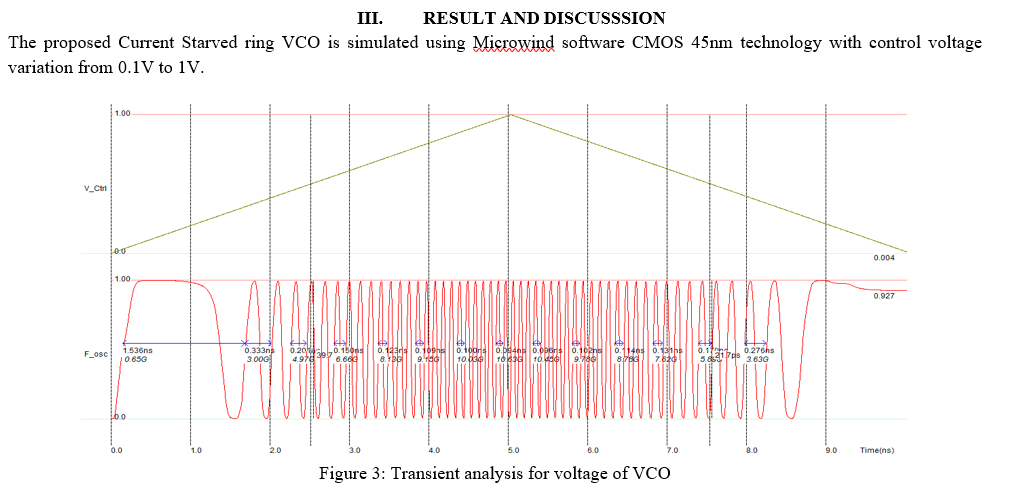
【高频领域挑战】:VCO设计在微波工程中的突破与机遇
# 摘要
本论文深入探讨了压控振荡器(VCO)的基础理论与核心设计原则,并在微波工程的应用技术中展开详细讨论。通过对VCO工作原理、关键性能指标以及在微波通信系统中的作用进行分析,本文揭示了VCO设计面临的主要挑战,并提出了相应的技术对策,包括频率稳定性提升和噪声性能优化的方法。此外,论文还探讨了VCO设计的实践方法、案例分析和故障诊断策略,最后对VCO设计的创新思路、新技术趋势及未来发展挑战
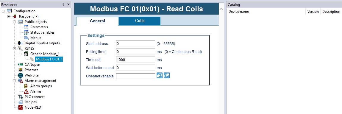
实现SUN2000数据采集:MODBUS编程实践,数据掌控不二法门
# 摘要
本文系统地介绍了MODBUS协议及其在数据采集中的应用。首先,概述了MODBUS协议的基本原理和数据采集的基础知识。随后,详细解析了MODBUS协议的工作原理、地址和数据模型以及通讯模式,包括RTU和ASCII模式的特性及应用。紧接着,通过Python语言的MODBUS库,展示了MODBUS数据读取和写入的编程实践,提供了具体的实现方法和异常管理策略。本文还结合SUN20
【性能调优秘籍】:深度解析sco506系统安装后的优化策略
# 摘要
本文对sco506系统的性能调优进行了全面的介绍,首先概述了性能调优的基本概念,并对sco506系统的核心组件进行了介绍。深入探讨了核心参数调整、磁盘I/O、网络性能调优等关键性能领域。此外,本文还揭示了高级性能调优技巧,包括CPU资源和内存管理,以及文件系统性能的调整。为确保系统的安全性能,文章详细讨论了安全策略、防火墙与入侵检测系统的配置,以及系统审计与日志管理的优化。最后,本文提供了系统监控与维护的
网络延迟不再难题:实验二中常见问题的快速解决之道
# 摘要
网络延迟是影响网络性能的重要因素,其成因复杂,涉及网络架构、传输协议、硬件设备等多个方面。本文系统分析了网络延迟的成因及其对网络通信的影响,并探讨了网络延迟的测量、监控与优化策略。通过对不同测量工具和监控方法的比较,提出了针对性的网络架构优化方案,包括硬件升级、协议配置调整和资源动态管理等。
期末考试必备:移动互联网商业模式与用户体验设计精讲

# 摘要
移动互联网的迅速发展带动了商业模式的创新,同时用户体验设计的重要性日益凸显。本文首先概述了移动互联网商业模式的基本概念,接着深入探讨用户体验设计的基础,包括用户体验的定义、重要性、用户研究方法和交互设计原则。文章重点分析了移动应用的交互设计和视觉设计原则,并提供了设计实践案例。之后,文章转向移动商业模式的构建与创新,探讨了商业模式框架
【多语言环境编码实践】:在各种语言环境下正确处理UTF-8与GB2312
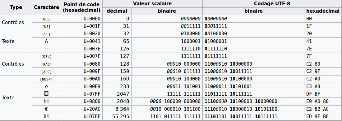
# 摘要
随着全球化的推进和互联网技术的发展,多语言环境下的编码问题变得日益重要。本文首先概述了编码基础与字符集,随后深入探讨了多语言环境所面临的编码挑战,包括字符编码的重要性、编码选择的考量以及编码转换的原则和方法。在此基础上,文章详细介绍了UTF-8和GB2312编码机制,并对两者进行了比较分析。此外,本文还分享了在不同编程语言中处理编码的实践技巧,
【数据库在人事管理系统中的应用】:理论与实践:专业解析
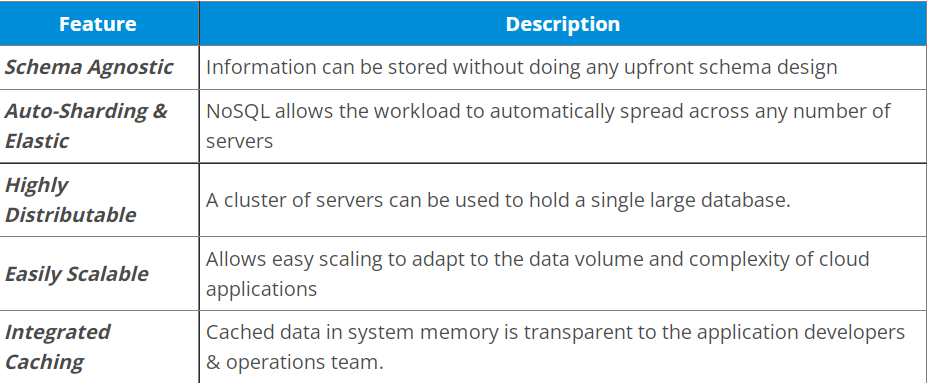
# 摘要
本文探讨了人事管理系统与数据库的紧密关系,分析了数据库设计的基础理论、规范化过程以及性能优化的实践策略。文中详细阐述了人事管理系统的数据库实现,包括表设计、视图、存储过程、触发器和事务处理机制。同时,本研究着重讨论了数据库的安全性问题,提出认证、授权、加密和备份等关键安全策略,以及维护和故障处理的最佳实践。最后,文章展望了人事管理系统的发展趋
【Docker MySQL故障诊断】:三步解决权限被拒难题
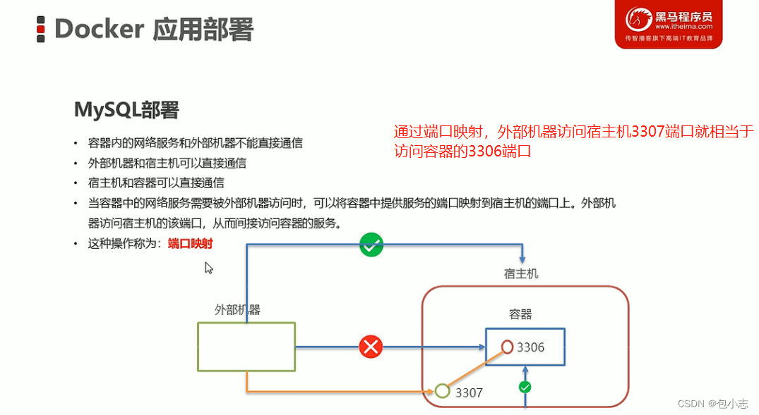
# 摘要
随着容器化技术的广泛应用,Docker已成为管理MySQL数据库的流行方式。本文旨在对Docker环境下MySQL权限问题进行系统的故障诊断概述,阐述了MySQL权限模型的基础理论和在Docker环境下的特殊性。通过理论与实践相结合,提出了诊断权限问题的流程和常见原因分析。本文还详细介绍了如何利用日志文件、配置检查以及命令行工具进行故障定位与修复,并探讨了权限被拒问题的解决策略和预防措施
资源上传下载、课程学习等过程中有任何疑问或建议,欢迎提出宝贵意见哦~我们会及时处理!
点击此处反馈


专栏目录
最低0.47元/天 解锁专栏
买1年送3月
百万级
高质量VIP文章无限畅学
千万级
优质资源任意下载
C知道
免费提问 ( 生成式Al产品 )