【Essentials of Deep Learning for Time Series Forecasting】: Tips and Advanced Applications of RNN

# Deep Learning Time Series Forecasting Essentials: Tips and Advanced Applications of RNN

## 1. Overview of Deep Learning and Time Series Forecasting

### 1.1 Introduction to Deep Learning Techniques
Deep learning, as a branch of the machine learning field, has become a core technology for handling complex data and pattern recognition. By simulating the working principles of the human brain's neural network, deep learning algorithms can automatically learn data representations and features without the need for manual feature design. This adaptive feature extraction capability has led to breakthroughs in deep learning in areas such as image recognition, speech processing, and natural language processing.

### 1.2 The Importance of Time Series Forecasting
Time series forecasting involves predicting future data points or trends based on historical data. This technology is widely applied in many fields, including finance, meteorology, economics, and energy. The purpose of time series forecasting is to learn patterns from past and present data to make reasonable predictions about future data within a certain period. Accurate time series forecasting is crucial for resource optimization, risk management, and decision-making.

### 1.3 Combining Deep Learning and Time Series Forecasting
Deep learning applications in time series forecasting, particularly through recurrent neural networks (RNNs) and their variants (such as LSTMs and GRUs), ***pared to traditional statistical methods, deep learning methods have unique advantages in nonlinear pattern recognition, thus providing more accurate predictions when dealing with complex, high-dimensional time series data.

## 2. Basic Principles and Structure of RNN Networks

### 2.1 Basics of Recurrent Neural Networks (RNN)

#### 2.1.1 How RNNs Work
Recurrent Neural Networks (RNNs) are a type of neural network designed for processing sequential data. In traditional feedforward neural networks, information flows in one direction, from the input layer to the hidden layer, and then to the output layer. The core feature of RNNs is their ability to use their memory to process sequential data, endowing the network with dynamic characteristics over time.

RNNs introduce a hidden state that allows the network to retain previous information and use it to influence subsequent outputs. This makes RNNs particularly suitable for tasks related to sequences, such as time series data, natural language, and speech.

At each time step, RNNs receive input data and the hidden state from the previous time step, then compute the current time step's hidden state and output. The output can be the classification result of the time step or a comprehensive representation of the entire sequence. The mathematical expression is as follows:

$$ h_t = f(h_{t-1}, x_t) $$

Here, $h_t$ is the hidden state of the current time step, $h_{t-1}$ is the hidden state of the previous time step, $x_t$ is the input of the current time step, and $f$ is a nonlinear activation function.

The hidden state maintains a "state" that can be understood as an encoding of the historical information of the sequence. This state update, i.e., the computation of the hidden layer, is achieved through recurrent connections, hence the name recurrent neural network.

#### 2.1.2 Comparison of RNNs with Other Neural Networks
Compared to traditional feedforward neural networks, the most significant difference with RNNs is their ability to process sequential data, ***

***pared to convolutional neural networks (CNNs), although CNNs can also process sequential data, their focus is on capturing local patterns through local receptive fields, while RNNs emphasize information transfer over time.

In addition to standard RNNs, there are several special recurrent network structures, such as Long Short-Term Memory (LSTM) networks and Gated Recurrent Units (GRUs), designed to solve the inherent problems of gradient vanishing and explosion in RNNs and to improve modeling capabilities for long-term dependencies. These improved RNN variants are more commonly used in practical applications due to their ability to more effectively train long sequence data.

### 2.2 RNN Mathematical Models and Computational Graphs

#### 2.2.1 Time Step Unfolding and the Vanishing Gradient Problem
In RNNs, due to the recurrent connections between hidden layers, RNNs can be viewed as multiple identical neural network layers connected in series over time. This structural feature leads to RNNs being unfolded into a very deep network during training, causing gradients to be propagated through many time steps during backpropagation. When the time steps are too long, it can result in the vanishing or exploding gradient problem.

The vanishing gradient problem refers to the phenomenon where gradients exponentially decrease in magnitude during backpropagation as the distance of propagation increases, causing the learning process to become very slow. The exploding gradient is the opposite, where gradients exponentially increase, causing unstable weight updates and even numerical overflow.

To address these issues, researchers have proposed various methods, such as using gradient clipping techniques to limit gradient size or using more complex, specially designed RNN variants like LSTMs and GRUs.

#### 2.2.2 Forward Propagation and Backpropagation
Forward propagation refers to the process in RNNs where, at each time step, input data is received and the hidden state is updated. This process continues until the sequence ends. During this process, the network generates output and passes the hidden state to the next time step.

Backpropagation is the process through time (Backpropagation Through Time, BPTT). In traditional backpropagation, error gradients are propagated downward through the network's layers. However, in RNNs, due to the network's unique structure, gradients must be propagated not only through the layers but also across the time dimension. When calculating the gradient for each time step, the gradient from the previous time step is accumulated. This step needs to be recursively repeated until the end of the entire sequence.

This process involves the chain rule, requiring the computation of the local gradient for each time step and combining it with the gradient from the previous time step to update the weights. This is achieved by solving partial derivatives and applying the chain rule, ultimately obtaining the gradient to be updated at each time step.

#### 2.2.3 RNN Variants: LSTMs and GRUs
Due to the gradient vanishing and exploding problems in standard RNNs, researchers have designed two special RNN structures, LSTMs and GRUs, to more effectively handle long-term dependencies.

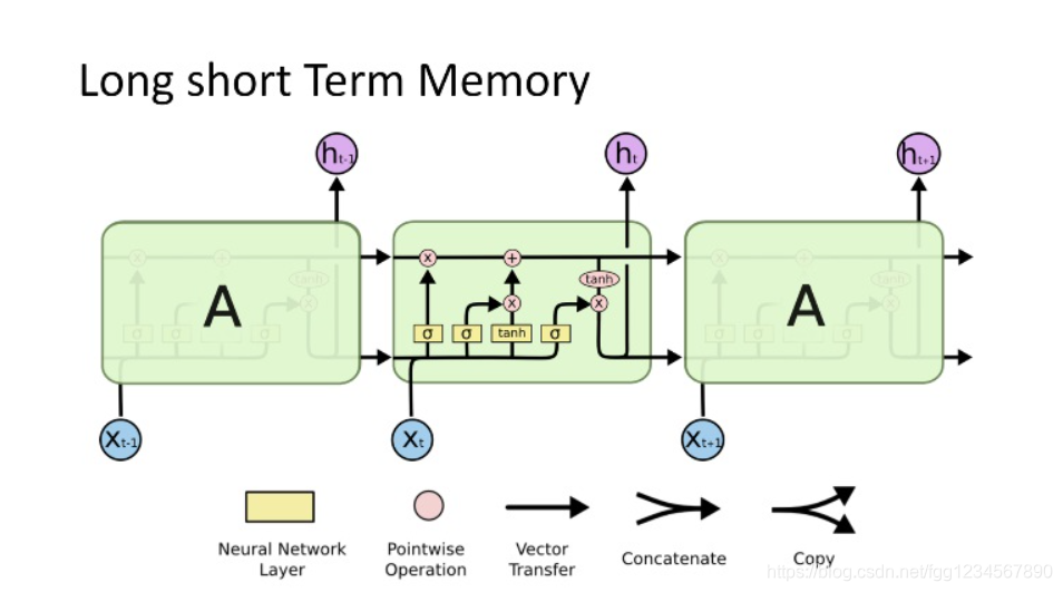
- **LSTM (Long Short-Term Memory):** The design concept of LSTMs is to introduce a gating mechanism at each time step that can decide what information to retain or forget. LSTMs have three gates: the forget gate (decides which information to discard), the input gate (decides which new information is saved into the state), and the output gate (decides the output of the next hidden state). With this design, LSTMs can preserve long-term dependency information in sequences while avoiding the vanishing gradient problem.

- **GRU (Gated Recurrent Unit):** GRUs can be seen as a simplified version of LSTMs. GRUs only use two gates: the reset gate (decides the extent to which new input is combined with old memory), and the update gate (decides how much old memory to retain). GRUs have a simpler structure than LSTMs but can still effectively handle long-term dependency issues.

These variants effectively solve the gradient problem through gating mechanisms and demonstrate outstanding performance in various sequence prediction tasks.

### Code Block Example: Forward Propagation of an RNN Model

Assuming we use the Keras library in Python to define a simple RNN model, here is a simplified code example:

from keras.models import Sequential
from keras.layers import SimpleRNN, Activation

# Create a model
model = Sequential()

# Add an RNN layer, assuming the input sequence length is 10 and the feature dimension is 50
model.add(SimpleRNN(64, input_shape=(10, 50), return_sequences=False))

# Add an activation layer
model.add(Activation('relu'))

# Compile the model
***pile(loss='mean_squared_error', optimizer='adam')

# Print model summary
model.summary()

#### Parameter Explanation:

- `Sequential()`: Creates a sequential model.
- `SimpleRNN(64, input_shape=(10, 50), return_sequences=False)`: Adds an RNN layer. Here, 64 neurons are used, and `input_shape` defines the shape of the input data (time step length of 10, feature dimension of 50). `return_sequences=False` indicates that only the last output of each time step is returned.
- `Activation('relu')`: Adds an activation layer using the ReLU activation function.
- `***pile(loss='mean_squared_error', optimizer='adam')`: Compiles the model, using mean squared error as the loss function and the Adam optimizer.

#### Logical Analysis:

In this simple RNN model, we define an input sequence with a length of 10 and a feature dimension of 50. The RNN layer generates output based on this data, and since `return_sequences=False`, we obtain the last output of each time step. The activation layer then applies the ReLU function to increase the model's nonlinear capability. Finally, we specify the loss function and optimizer by compiling the model.

In practical applications, LSTMs or GRUs are often used to build models because they perform better in many tasks, especially when seq