矩阵运算在运筹学中的广泛应用：优化决策的数学工具

# 1. 矩阵运算的基本原理**

矩阵运算是一种数学运算，它涉及到对包含数字或其他数学对象的矩形数组（矩阵）进行操作。矩阵运算在运筹学中有着广泛的应用，因为它可以有效地表示和解决复杂的问题。

矩阵运算的基本操作包括加法、减法、乘法和转置。矩阵加法和减法是按元素进行的，而矩阵乘法则涉及到矩阵元素的乘积和求和。矩阵转置是将矩阵的行和列交换。这些基本操作可以组合起来执行更复杂的运算，例如求逆、求特征值和特征向量。

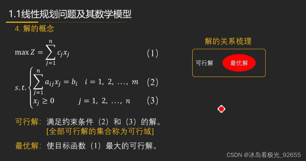
# 2.1 线性规划

### 2.1.1 线性规划模型的建立

线性规划模型的建立包括以下步骤：

1. **确定决策变量：**决策变量是需要在模型中求解的未知数，通常表示为 x1、x2、...。
2. **建立目标函数：**目标函数表示需要最大化或最小化的目标，通常是一个线性函数，如 max z = c1x1 + c2x2 + ... + cnxn。
3. **建立约束条件：**约束条件限制决策变量的值，通常是一组线性不等式或等式，如 a1x1 + a2x2 + ... + anxn ≤ b。

### 2.1.2 线性规划的求解方法

线性规划的求解方法主要有两种：

1. **单纯形法：**单纯形法是一种迭代算法，从一个可行解开始，通过一系列步骤逐步逼近最优解。
2. **内点法：**内点法是一种直接求解法，通过在可行域内部迭代，直接找到最优解。

**代码示例：**

import numpy as np
from scipy.optimize import linprog

# 目标函数系数
c = np.array([1, 2])

# 约束条件系数矩阵
A = np.array([[1, 1], [2, 3]])

# 约束条件右端值
b = np.array([5, 8])

# 求解线性规划
res = linprog(c, A_ub=A, b_ub=b)

# 打印最优解
print("最优解：", res.x)
print("最优目标值：", res.fun)

**逻辑分析：**

* `linprog` 函数用于求解线性规划问题。
* `c` 参数指定目标函数系数。
* `A_ub` 和 `b_ub` 参数指定约束条件系数矩阵和右端值。
* `res.x` 属性返回最优解。
* `res.fun` 属性返回最优目标值。

# 3. 矩阵运算在运筹学中的实践

### 3.1 物流优化

#### 3.1.1 物流网络的建立

物流网络的建立是物流优化中的重要环节。它涉及到仓库、配送中心、运输工具等多个要素的规划。矩阵运算可以帮助我们建立一个高效的物流网络，以最小化成本和时间。

**建立物流网络的步骤：**

1. **确定需求点和供应点：**确定需要接收货物的地点（需求点）和提供货物的仓库或配送中心（供应点）。
2. **建立距离矩阵：**计算需求点和供应点之间的距离，形成一个距离矩阵。
3. **建立运输成本矩阵：**计算不同运输方式下，从供应点到需求点的运输成本，形成一个运输成本矩阵。
4. **建立网络流模型：**使用线性规划模型，建立一个网络流模型来优化物流网络。该模型的目标函数是最小化总运输成本。
5. **求解网络流模型：**使用线性规划求解器，求解网络流模型，得到最优的物流网络方案。

**代码示例：**

import numpy as np
from scipy.optimize import linprog

# 需求点和供应点
demand_points = ["A", "B", "C"]
supply_points = ["S1", "S2"]

# 距离矩阵
distance_matrix = np.array([[0, 10, 15], [10, 0, 20], [15, 20, 0]])

# 运输成本矩阵
cost_matrix = np.array([[5, 10], [10, 5], [15, 15]