Multilayer Perceptron (MLP) Image Recognition in Practice: From Beginner to Expert, The Advanced Path to Image Recognition
发布时间: 2024-09-15 07:57:26 阅读量: 27 订阅数: 31 

multilayer-perceptron-in-c:多层感知器在C语言中的实现
# 1. Multilayer Perceptron (MLP) Fundamentals
A Multilayer Perceptron (MLP) is a type of feedforward artificial neural network that is widely used in fields such as image recognition. It consists of multiple fully connected layers, where each neuron in one layer is connected to every neuron in the following layer.
The learning algorithm for MLPs often utilizes the backpropagation algorithm. This algorithm minimizes the loss function by computing the error gradient and updating the weights. The weight update formula is as follows:
```
w_new = w_old - α * ∂L/∂w
```
Where:
* `w_new` is the updated weight.
* `w_old` is the weight before the update.
* `α` is the learning rate.
* `∂L/∂w` is the partial derivative of the loss function with respect to the weight.
# 2. MLP Theory for Image Recognition
### 2.1 MLP Model Structure and Principles
#### 2.1.1 MLP Network Structure
A Multilayer Perceptron (MLP) is a feedforward neural network composed of multiple layers of nodes (neurons). These nodes are arranged in layers, with each layer connected to the one above and the one below. The structure of an MLP can be represented as:
```
Input Layer -> Hidden Layer 1 -> Hidden Layer 2 -> ... -> Output Layer
```
The input layer receives input data, and the output layer produces predictions. The hidden layers perform nonlinear transformations between the input and output, allowing the MLP to learn complex patterns.
#### 2.1.2 MLP Learning Algorithm
MLPs use the backpropagation algorithm for training. The algorithm updates network weights through the following steps:
1. **Forward Propagation:** Input data is passed through the network, from the input layer to the output layer.
2. **Compute Error:** The error between the predictions of the output layer and the true labels is calculated as the loss function.
3. **Backward Propagation:** The error is propagated back through the network to calculate the gradient for each weight.
4. **Weight Update:** Weights are updated using the gradient descent algorithm to minimize the loss function.
### 2.2 Principles of Image Recognition
#### 2.2.1 Image Feature Extraction
Image recognition involves extracting features from images that can be used to classify them. MLPs can utilize techniques such as Convolutional Neural Networks (CNNs) ***Ns use filters to slide over the image, extracting features such as edges, textures, and shapes.
#### 2.2.2 Image Classification
After feature extraction, MLPs use a classifier to categorize images. Classifiers typically involve a softmax function, which maps the feature vector to a probability distribution, representing the probability of the image belonging to each category.
```
softmax(x) = exp(x) / sum(exp(x))
```
Where `x` is the feature vector, `exp` is the exponential function, and `sum` is the summation function.
# 3. MLP Practice in Image Recognition
### 3.1 Data Preprocessing
#### 3.1.1 Image Data Acquisition and Loading
**Acquiring Image Data**
Acquiring image data is the first step in image recognition tasks. Image data can be obtained from various sources, such as:
- Public datasets (e.g., MNIST, CIFAR-10)
- Web scraping
- Capturing or collecting images personally
**Loading Image Data**
After acquiring image data, ***mon image loading libraries include:
- OpenCV
- Pillow
- Matplotlib
**Code Block: Loading Image Data**
```python
import cv2
# Loading an image from a file
image = cv2.imread('image.jpg')
# Converting the image to a NumPy array
image_array = cv2.cvtColor(image, cv2.COLOR_BGR2RGB)
```
**Logical Analysis:**
* The `cv2.imread()` function reads an image from a file and converts it into BGR (Blue, Green, Red) format.
* The `cv2.cvtColor()` function converts the image from BGR format to RGB (Red, Green, Blue) format, which is used by most deep learning frameworks.
#### 3.1.2 Image Preprocessing and Augmentation
**Image Preprocessing**
***mon preprocessing steps include:
- Resizing
- Normalization
- Data augmentation
**Image Augmentation**
***mon augmentation techniques include:
- Flipping
- Rotation
- Cropping
- Adding noise
**Code Block: Image Preprocessing and Augmentation**
```python
import numpy as np
# Resizing the image
image_resized = cv2.resize(image_array, (224, 224))
# Normalizing the image
image_normalized = image_resized / 255.0
# Flipping the image
image_flipped = cv2.flip(image_normalized, 1)
# Rotating the image
image_rotated = cv2.rotate(image_normalized, cv2.ROTATE_90_CLOCKWISE)
```
**Logical Analysis:**
* The `cv2.resize()` function adjusts the size of the image.
* The `image_normalized` normalizes the image pixel values to the range [0, 1].
* The `cv2.flip()` function horizontally flips the image.
* The `cv2.rotate()` function rotates the image 90 degrees clockwise.
### 3.2 Model Training and Evaluation
#### 3.2.1 Model Construction and Parameter Settings
**Model Construction**
The construction of an MLP image recognition model includes the following steps:
1. Defining the input layer (image pixels)
2. Defining the hidden layers (multiple fully connected layers)
3. Defining the output layer (image categories)
**Parameter Settings**
Parameters for an MLP model include:
- Number of hidden layers
- Number of neurons in each hidden layer
- Activation function
- Optimization algorithm
- Learning rate
**Code Block: Model Construction and Parameter Settings**
```python
import tensorflow as tf
# Defining the input layer
input_layer = tf.keras.layers.Input(shape=(224, 224, 3))
# Defining the hidden layers
hidden_layer_1 = tf.keras.layers.Dense(512, activation='relu')(input_layer)
hidden_layer_2 = tf.keras.layers.Dense(256, activation='relu')(hidden_layer_1)
# Defining the output layer
output_layer = tf.keras.layers.Dense(10, activation='softmax')(hidden_layer_2)
# Defining the model
model = tf.keras.Model(input_layer, output_layer)
# ***
***pile(optimizer='adam', loss='categorical_crossentropy', metrics=['accuracy'])
```
**Logical Analysis:**
* The `tf.keras.layers.Input()` function defines the input layer, with a shape of (224, 224, 3), indicating the size and number of channels of the input images.
* The `tf.keras.layers.Dense()` function defines the hidden layers; the first hidden layer has 512 neurons with a ReLU activation function. The second hidden layer has 256 neurons, also with a ReLU activation function.
* The `tf.keras.layers.Dense()` function defines the output layer, with 10 neurons and a softmax activation function, suitable for multi-class classification tasks.
* The `***pile()` function compiles the model, specifying the optimizer, loss function, and evaluation metrics.
#### 3.2.2 Model Training and Hyperparameter Optimization
**Model Training**
Model training is the process of updating model parameters using training data. The training process includes:
1. Forward propagation: ***
***puting loss: Comparing the difference between predicted and actual values.
3. Backward propagation: Calculating the gradient of the loss function with respect to the model parameters.
4. Updating parameters: Using an optimization algorithm to update the model parameters.
**Hyperparameter Optimization**
Hyperparameter optimization is the process of adjusting model hyperparameters (e.g., learning rate, number of hidden layers) ***mon optimization methods include:
- Grid Search
- Random Search
- Bayesian Optimization
**Code Block: Model Training and Hyperparameter Optimization**
```python
# Preparing training data
train_data = ...
# Training the model
model.fit(train_data, epochs=10)
# Hyperparameter optimization
from sklearn.model_selection import GridSearchCV
param_grid = {
'learning_rate': [0.001, 0.0001],
'hidden_layer_1': [128, 256],
'hidden_layer_2': [64, 128]
}
grid_search = GridSearchCV(model, param_grid, cv=5)
grid_search.fit(train_data, epochs=10)
```
**Logical Analysis:**
* The `model.fit()` function trains the model, specifying the training data and the number of epochs.
* The `GridSearchCV` performs hyperparameter optimization, trying different combinations of hyperparameters and selecting the best-performing combination.
#### 3.2.3 Model Evaluation and Performance Analysis
**Model Evaluation**
Model evaluation is the process of assessing model performance using validation or test data. Evaluation metrics include:
- Accuracy
- Recall
- F1 Score
- Confusion Matrix
**Performance Analysis**
Performance analysis is the process of analyzing the model evaluation results to determine the strengths and weaknesses of the model. Performance analysis can help improve the model and increase its generalization capabilities.
**Code Block: Model Evaluation and Performance Analysis**
```python
# Preparing validation data
validation_data = ...
# Evaluating the model
loss, accuracy = model.evaluate(validation_data)
# Plotting the confusion matrix
import seaborn as sns
sns.heatmap(confusion_matrix(y_true, y_pred), annot=True)
```
**Logical Analysis:**
* The `model.evaluate()` function evaluates the model, returning the loss value and accuracy.
* The `confusion_matrix()` function calculates the confusion matrix, showing the prediction results of the model across different classes.
# 4. Advanced MLP Image Recognition
### 4.1 Model Optimization and Improvement
#### 4.1.1 Activation Functions and Optimization Algorithms
**Activation Functions**
***mon activation functions include:
- **Sigmoid Function:** `f(x) = 1 / (1 + e^(-x))`
- **Tanh Function:** `f(x) = (e^x - e^(-x)) / (e^x + e^(-x))`
- **ReLU Function:** `f(x) = max(0, x)`
Different activation functions have different nonlinear characteristics, which can significantly affect the performance of the model.
**Optimization Algorithms**
Op***mon optimization algorithms include:
- **Gradient Descent:** `w = w - lr * ∇L(w)`
- **Momentum:** `v = β * v + (1 - β) * ∇L(w)`
- **RMSprop:** `s = β * s + (1 - β) * (∇L(w))^2`
Different optimization algorithms have different convergence speeds and stability.
#### 4.1.2 Regularization and Overfitting Handling
**Regularization**
Regularization is a techn***mon regularization methods include:
- **L1 Regularization:** `L1(w) = ∑|w|`
- **L2 Regularization:** `L2(w) = ∑w^2`
**Overfitting Handling**
Overfitting occurs when a model performs well on the training set but poorly on new data. Methods to handle overfitting include:
- **Data Augmentation:** Increase the size of the training dataset by operations such as rotation, cropping, and flipping.
- **Dropout:** Randomly drop neurons during training to prevent the model from relying too much on specific features.
- **Early Stopping:** Stop training when the model's performance on the validation set no longer improves.
### 4.2 Application Scenarios and Extensions
#### 4.2.1 Object Detection and Segmentation
MLPs can be used for object detection and segmentation tasks. Object detection involves identifying and locating targets within an image. Segmentation involves separating the objects in an image from the background.
#### 4.2.2 Face Recognition and Expression Analysis
MLPs can be applied to face recognition and expression analysis tasks. Face recognition involves identifying and determining the identity of faces in images. Expression analysis involves identifying the expressions of people in images.
**Code Example:**
```python
import tensorflow as tf
# Building an MLP model
model = tf.keras.models.Sequential([
tf.keras.layers.Dense(128, activation='relu', input_shape=(784,)),
tf.keras.layers.Dense(64, activation='relu'),
tf.keras.layers.Dense(10, activation='softmax')
])
# ***
***pile(optimizer='adam', loss='sparse_categorical_crossentropy', metrics=['accuracy'])
# Training the model
model.fit(x_train, y_train, epochs=10)
# Evaluating the model
model.evaluate(x_test, y_test)
```
**Logical Analysis of the Code:**
- The `***pile()` method compiles the model, specifying the optimizer, loss function, and evaluation metrics.
- The `model.fit()` method trains the model, specifying the training data and the number of epochs.
- The `model.evaluate()` method evaluates the model, specifying the test data and evaluation metrics.
**Parameter Explanation:**
- `optimizer`: The optimization algorithm, such as 'adam'.
- `loss`: The loss function, such as 'sparse_categorical_crossentropy'.
- `metrics`: Evaluation metrics, such as 'accuracy'.
- `epochs`: The number of training epochs.
# 5. MLP Image Recognition Case Studies
### 5.1 Handwritten Digit Recognition
#### 5.1.1 Dataset Introduction and Loading
Handwritten digit recognition is a classic task in the field of image recognition. We will use the MNIST dataset, which is a widely used dataset containing 70,000 handwritten digit images. The dataset is divided into a training set and a test set, with 60,000 and 10,000 images respectively.
**Code Block: Loading the MNIST Dataset**
```python
import tensorflow as tf
# Loading the MNIST dataset
(x_train, y_train), (x_test, y_test) = tf.keras.datasets.mnist.load_data()
# Normalizing the image pixel values
x_train, x_test = x_train / 255.0, x_test / 255.0
# Converting labels to one-hot encoding
y_train = tf.keras.utils.to_categorical(y_train, 10)
y_test = tf.keras.utils.to_categorical(y_test, 10)
```
#### 5.1.2 Model Construction and Training
We will use a simple MLP model to perform the handwritten digit recognition task. The model will include an input layer, a hidden layer, and an output layer.
**Code Block: Building the MLP Model**
```python
# Building an MLP model
model = tf.keras.Sequential([
tf.keras.layers.Flatten(input_shape=(28, 28)),
tf.keras.layers.Dense(128, activation='relu'),
tf.keras.layers.Dense(10, activation='softmax')
])
```
**Code Block: Compiling and Training the Model**
```python
# ***
***pile(optimizer='adam',
loss='categorical_crossentropy',
metrics=['accuracy'])
# Training the model
model.fit(x_train, y_train, epochs=10)
```
#### 5.1.3 Model Evaluation and Result Analysis
After training the model, we will evaluate its performance using the test set.
**Code Block: Evaluating the Model**
```python
# Evaluating the model
loss, accuracy = model.evaluate(x_test, y_test)
# Printing the evaluation results
print('Test loss:', loss)
print('Test accuracy:', accuracy)
```
### 5.2 Image Classification
#### 5.2.1 Dataset Introduction and Loading
We will use the CIFAR-10 dataset, which is an image classification dataset containing 60,000 32x32 color images. The dataset is divided into a training set and a test set, with 50,000 and 10,000 images respectively.
**Code Block: Loading the CIFAR-10 Dataset**
```python
import tensorflow as tf
# Loading the CIFAR-10 dataset
(x_train, y_train), (x_test, y_test) = tf.keras.datasets.cifar10.load_data()
# Normalizing the image pixel values
x_train, x_test = x_train / 255.0, x_test / 255.0
# Converting labels to one-hot encoding
y_train = tf.keras.utils.to_categorical(y_train, 10)
y_test = tf.keras.utils.to_categorical(y_test, 10)
```
#### 5.2.2 Model Construction and Training
We will use a more complex MLP model to perform the image classification task. The model will include multiple hidden layers and an output layer.
**Code Block: Building the MLP Model**
```python
# Building an MLP model
model = tf.keras.Sequential([
tf.keras.layers.Flatten(input_shape=(32, 32, 3)),
tf.keras.layers.Dense(512, activation='relu'),
tf.keras.layers.Dense(256, activation='relu'),
tf.keras.layers.Dense(10, activation='softmax')
])
```
**Code Block: Compiling and Training the Model**
```python
# ***
***pile(optimizer='adam',
loss='categorical_crossentropy',
metrics=['accuracy'])
# Training the model
model.fit(x_train, y_train, epochs=10)
```
#### 5.2.3 Model Evaluation and Result Analysis
After training the model, we will evaluate its performance using the test set.
**Code Block: Evaluating the Model**
```python
# Evaluating the model
loss, accuracy = model.evaluate(x_test, y_test)
# Printing the evaluation results
print('Test loss:', loss)
print('Test accuracy:', accuracy)
```
# 6. Future Developments of MLP Image Recognition
### 6.1 Deep Learning and Transfer Learning
In recent years, deep learning has achieved tremendous success in the field of image recognition. Deep learning models, such as Convolutional Neural Networks (CNNs), are capable of automatically learning complex features from images, thus achieving higher recognition accuracy.
Transfer learning is a technique that involves applying pre-trained models to new tasks. Through transfer learning, we can utilize the features extracted by pre-trained models to train new MLP models, thereby enhancing model performance and training efficiency.
### ***
***puter vision aims to enable computers to understand and interpret information within images. As artificial intelligence (AI) technology continues to advance, ***
** technology can endow computers with the ability to recognize and understand complex semantic information within images. For example, AI-driven image recognition systems can identify objects, scenes, emotions, and actions within images. These capabilities are crucial for applications such as autonomous driving, face recognition, and medical diagnosis.
### Code Example
The following code demonstrates how to use transfer learning to train an MLP image recognition model:
```python
import tensorflow as tf
# Loading the pre-trained VGG16 model
vgg16 = tf.keras.applications.VGG16(include_top=False, weights='imagenet')
# Freezing the weights of the VGG16 model
vgg16.trainable = False
# Creating an MLP model
mlp = tf.keras.Sequential([
tf.keras.layers.Flatten(input_shape=(224, 224, 3)),
tf.keras.layers.Dense(512, activation='relu'),
tf.keras.layers.Dense(256, activation='relu'),
tf.keras.layers.Dense(10, activation='softmax')
])
# Building the transfer learning model
transfer_model = tf.keras.Sequential([
vgg16,
mlp
])
# Compiling the model
transfer_***pile(optimizer='adam', loss='sparse_categorical_crossentropy', metrics=['accuracy'])
# Training the model
transfer_model.fit(train_data, train_labels, epochs=10)
```
### Conclusion
MLP image recognition technology is continuously advancing. The application of deep learning, transfer learning, and AI technology will further propel its development. In the future, image recognition technology will continue to play a significant role in various fields, bringing more convenience and possibilities to human life.

 百万级
高质量VIP文章无限畅学
百万级
高质量VIP文章无限畅学
 千万级
优质资源任意下载
千万级
优质资源任意下载
 C知道
免费提问 ( 生成式Al产品 )
C知道
免费提问 ( 生成式Al产品 )
0
0
相关推荐

专栏目录
最低0.47元/天 解锁专栏
买1年送3月
百万级
高质量VIP文章无限畅学
千万级
优质资源任意下载
C知道
免费提问 ( 生成式Al产品 )
最新推荐
【自定义你的C#打印世界】:高级技巧揭秘,满足所有打印需求
# 摘要
本文详细探讨了C#打印机制的底层原理及其核心组件,分析了C#打印世界的关键技术,包括System.Drawing.Printing命名空间和PrinterSettings类的使用,以及PageSettings和PrintDocument类在打印操作API中的作用。本文还介绍了如何设计C#打印模板,进行打印流程的高级优化,并探讨了C#打印解决方案的跨平台实现。通过C#打印实践案例解析,本文提供了在桌面和网络应用中实现打印功能的指导,并讨论了相关测试与维护策略。最终,本文展望了云计算与C#打印技术结合的未来趋势,以及AI与机器学习在打印领域的创新应用,强调了开源社区对技术进步的贡献。
【自动化调度系统入门】:零基础理解程序化操作
# 摘要
自动化调度系统是现代信息技术中的核心组件,它负责根据预定义的规则和条件自动安排和管理任务和资源。本文从自动化调度系统的基本概念出发,详细介绍了其理论基础,包括工作原理、关键技术、设计原则以及日常管理和维护。进一步,本文探讨了如何在不同行业和领域内搭建和优化自动化调度系统的实践环境,并分析了未来技术趋势对自动化调度系统的影响。文章通过案例分析展示了自动化调度系统在提升企业流程效率、成本控制
Android中的权限管理:IMEI码获取的安全指南
# 摘要
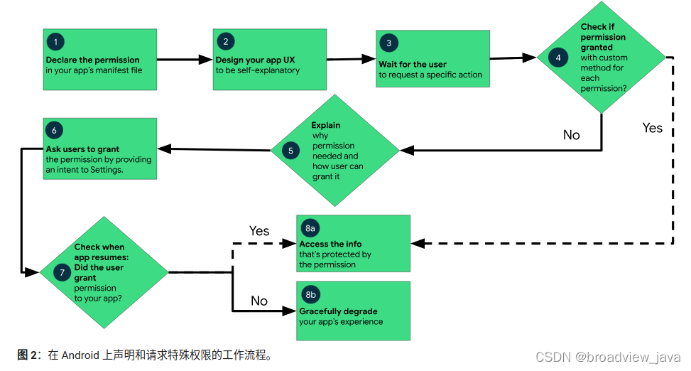
随着移动设备的普及,Android权限管理和IMEI码在系统安全与隐私保护方面扮演着重要角色。本文从Android权限管理概述出发,详细介绍IMEI码的基础知识及其在Android系统中的访问限制,以及获取IMEI码的理论基础和实践操作。同时,本文强调了保护用户隐私的重要性,并提供了安全性和隐私保护的实践措施。最后,文章展望了Android权限管理的未来趋势,并探讨了最佳实践,旨在帮助开发者构建更加安全可靠的
DW1000无线通信模块全方位攻略:从入门到精通的终极指南
# 摘要
本文旨在全面介绍DW1000无线通信模块的理论基础、配置、调试以及应用实践。首先,概述了DW1000模块的架构和工作机制,并对其通信协议及其硬件接口进行了详细解析。接着,文章深入探讨了模块配置与调试的具体方法,包括参数设置和网络连接建立。在应用实践方面,展示了如何利用DW1000实现精确的距离测量、构建低功耗局域网以及与微控制器集成。最后,本文探讨了DW1000模块的高级应用,包括最新通信技术和安全机制,以及对未来技术趋势和扩展性的分析。
# 关键字
DW1000模块;无线通信;通信协议;硬件接口;配置调试;距离测量;低功耗网络;数据加密;安全机制;技术前景
参考资源链接:[DW
【LaTeX符号大师课】:精通特殊符号的10个秘诀
# 摘要
LaTeX作为一个广泛使用的排版系统,特别在数学和科技文档排版中占有一席之地。本文全面介绍了LaTeX符号的使用,从基础的数学符号概述到符号的高级应用和管理实战演练。文章首先对LaTeX中的数学符号及其排版技巧进行了深入讲解,并探讨了特殊字符和图表结合时符号的应用。随后,文章重点介绍了如何通过宏包和定制化命令扩展符号的使用范围,并实现符号的自动化和跨文档复用。最后,通过实战演练,本文展示了如何在实际文档中综合应用这些符号排版技巧,并提出了符号排版的优化与维护建议。本文旨在为LaTeX用户提供一套完整的学习资源,以提升他们在符号排版方面的专业技能。
# 关键字
LaTeX符号;数学模
内存泄漏不再怕:手把手教你从新手到专家的内存管理技巧
# 摘要
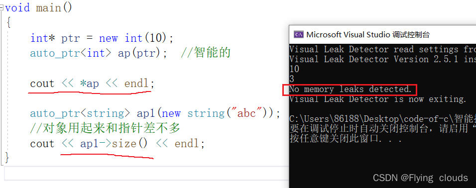
内存泄漏是影响程序性能和稳定性的关键因素,本文旨在深入探讨内存泄漏的原理及影响,并提供检测、诊断和防御策略。首先介绍内存泄漏的基本概念、类型及其对程序性能和稳定性的影响。随后,文章详细探讨了检测内存泄漏的工具和方法,并通过案例展示了诊断过程。在防御策略方面,本文强调编写内存安全的代码,使用智能指针和内存池等技术,以及探讨了优化内存管理策略,包括内存分配和释放的优化以及内存压缩技术的应用。本文不
【确保支付回调原子性】:C#后台事务处理与数据库操作的集成技巧
# 摘要
本文深入探讨了事务处理与数据库操作在C#环境中的应用与优化,从基础概念到高级策略。首先介绍了事务处理的基础知识和C#的事务处理机制,包括ACID属性和TransactionScope类的应用。随后,文章详细阐述了C#中事务处理的高级特性,如分布式事务和隔离级别对性能的影响,并探讨了性能优化的方法。第三章聚焦于C#集成实践中的数据库操作,涵盖ADO.NET和Entity Framework的事务处理集成,以及高效的数据库操作策略。第四章讨论了支付系统中保证事务原子性的具体策略和实践。最后,文章展望了分布式系统和异构数据库系统中事务处理的未来趋势,包括云原生事务处理和使用AI技术优化事务
E5071C与EMC测试:流程、合规性与实战分析(测试无盲区)
# 摘要
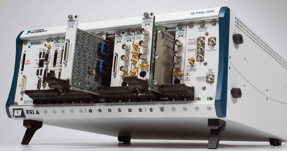
本文全面介绍了EMC测试的流程和E5071C矢量网络分析仪在其中的应用。首先概述了EMC测试的基本概念、重要性以及相关的国际标准。接着详细探讨了测试流程,包括理论基础、标准合规性评估、测试环境和设备准备。文章深入分析了E5071C性能特点和实际操作指南,并通过实战案例来展现其在EMC测试中的应用与优势。最后,探讨了未来EMC测试技术的发展趋势,包括智能化和自动化测试
资源上传下载、课程学习等过程中有任何疑问或建议,欢迎提出宝贵意见哦~我们会及时处理!
点击此处反馈


专栏目录
最低0.47元/天 解锁专栏
买1年送3月
百万级
高质量VIP文章无限畅学
千万级
优质资源任意下载
C知道
免费提问 ( 生成式Al产品 )