In-depth Analysis of Autocorrelation Function: A Comprehensive Interpretation of Theory and Applications
发布时间: 2024-09-15 17:55:33 阅读量: 38 订阅数: 29 

matlab自相关代码-stentor-cilia-autocorrelation:支架或纤毛自相关
# 1. Theoretical Foundation of the Autocorrelation Function
The autocorrelation function (ACF) is a mathematical tool used to measure the correlation between observations in a time series that are separated by a certain time interval. It is widely used in fields such as signal processing, image processing, and time series analysis.
The definition of the autocorrelation function is as follows:
```
ACF(k) = Cov(X(t), X(t+k)) / Var(X(t))
```
Where:
* `X(t)` is the time series
* `k` is the time interval
* `Cov()` is the covariance
* `Var()` is the variance
# 2. Calculation Methods of the Autocorrelation Function
There are mainly three methods to calculate the autocorrelation function:
### 2.1 Direct Calculation Method
The direct calculation method is the most intuitive approach, with the formula as follows:
```python
def autocorr_direct(x):
"""
Direct calculation of the autocorrelation function
Args:
x: Input signal
Returns:
Autocorrelation function
"""
n = len(x)
result = np.zeros(n)
for i in range(n):
for j in range(n - i):
result[i] += x[j] * x[j + i]
return result / n
```
**Line-by-line code logic explanation:**
* Line 1: Define the `autocorr_direct` function to directly calculate the autocorrelation function.
* Line 3: Get the length `n` of the input signal `x`.
* Line 4: Initialize the autocorrelation function result array `result`, with a size of `n`.
* Line 5-7: Use a nested loop to traverse the signal and calculate the autocorrelation value for each time shift `i`.
* Line 8: Divide the autocorrelation value by the signal length `n` to obtain the normalized autocorrelation function.
### 2.2 Fourier Transform Method
The Fourier transform method utilizes the properties of the Fourier transform to calculate the autocorrelation function, with the formula as follows:
```python
def autocorr_fft(x):
"""
Fourier transform method for calculating the autocorrelation function
Args:
x: Input signal
Returns:
Autocorrelation function
"""
n = len(x)
X = np.fft.fft(x)
result = np.fft.ifft(np.multiply(X, np.conj(X)))
return np.real(result)[:n]
```
**Line-by-line code logic explanation:**
* Line 1: Define the `autocorr_fft` function, which uses the Fourier transform method to calculate the autocorrelation function.
* Line 3: Get the length `n` of the input signal `x`.
* Line 4: Perform a Fourier transform on the signal `x` to obtain the frequency domain signal `X`.
* Line 5: Calculate the product of the frequency domain signal `X` and its conjugate `np.conj(X)`.
* Line 6: Perform an inverse Fourier transform on the product to obtain the autocorrelation function in the time domain.
* Line 7: Take the first `n` elements of the inverse Fourier transform result to obtain the normalized autocorrelation function.
### 2.3 Correlation Matrix Method
The correlation matrix method uses the properties of the correlation matrix to calculate the autocorrelation function, with the steps as follows:
**Step 1: Construct the correlation matrix**
```python
def corr_matrix(x):
"""
Construct the correlation matrix
Args:
x: Input signal
Returns:
Correlation matrix
"""
n = len(x)
C = np.zeros((n, n))
for i in range(n):
for j in range(n):
C[i, j] = np.corrcoef(x[i:], x[j:])[0, 1]
return C
```
**Step 2: Extract the autocorrelation function**
```python
def autocorr_matrix(x):
"""
Correlation matrix method for calculating the autocorrelation function
Args:
x: Input signal
Returns:
Autocorrelation function
"""
C = corr_matrix(x)
return C.diagonal()
```
**Line-by-line code logic explanation:**
* Line 1: Define the `corr_matrix` function, which is used to construct the correlation matrix.
* Line 3: Get the length `n` of the input signal `x`.
* Line 4: Initialize the correlation matrix `C`, with a size of `n x n`.
* Line 5-7: Use a nested loop to traverse the signal and calculate the correlation coefficient between each time shift `i` and `j`.
* Line 1: Define the `autocorr_matrix` function, which uses the correlation matrix method to calculate the autocorrelation function.
* Line 3: Call the `corr_matrix` function to construct the correlation matrix `C`.
* Line 4: Extract the diagonal elements of the correlation matrix to obtain the autocorrelation function.
# 3. Properties of the Autocorrelation Function
### 3.1 Symmetry
The autocorrelation function has symmetry, that is, for any time shift $\tau$, the following holds:
```
R_x(\tau) = R_x(-\tau)
```
**Proof:**
According to the definition of the autocorrelation function, we have:
```
R_x(\tau) = E[X(t)X(t+\tau)]
```
By substituting $t$ with $t-\tau$, we get:
```
R_x(-\tau) = E[X(t-\tau)X(t)]
```
Since $X(t)$ is a stationary random process, its statistical characteristics are time-invariant, hence:
```
E[X(t)X(t+\tau)] = E[X(t-\tau)X(t)]
```
Thus:
```
R_x(\tau) = R_x(-\tau)
```
**Corollary:**
The symmetry of the autocorrelation function indicates that, for a stationary random process, it is an even function in the time domain.
### 3.2 Non-negativity
The autocorrelation function is non-negative, that is, for any time shift $\tau$, the following holds:
```
R_x(\tau) ≥ 0
```
**Proof:**
According to the definition of the autocorrelation function, we have:
```
R_x(\tau) = E[X(t)X(t+\tau)]
```
Since $X(t)$ and $X(t+\tau)$ are stationary random processes with zero mean, we have:
```
E[X(t)X(t+\tau)] = E[(X(t) - E[X(t)])(X(t+\tau) - E[X(t+\tau)])]
```
Expanding and rearranging, we get:
```
R_x(\tau) = E[X(t)^2] + E[X(t+\tau)^2] - 2E[X(t)X(t+\tau)]
```
Since $X(t)$ and $X(t+\tau)$ are stationary random processes with equal variance, we have:
```
R_x(\tau) = 2\sigma^2 - 2E[X(t)X(t+\tau)]
```
Where $\sigma^2$ is the variance of $X(t)$.
Since $X(t)$ and $X(t+\tau)$ are stationary random processes, their covariance equals the autocorrelation function, thus:
```
R_x(\tau) = 2\sigma^2 - 2R_x(\tau)
```
Rearranging, we get:
```
R_x(\tau) = \sigma^2
```
Since $\sigma^2$ is non-negative, $R_x(\tau)$ is also non-negative.
**Corollary:**
The non-negativity of the autocorrelation function indicates that, for a stationary random process, it is the square root function of the autocorrelation function in the time domain.
### 3.3 Peak Characteristics
The autocorrelation function reaches its maximum value at a time shift $\tau = 0$, that is:
```
R_x(0) = max{|R_x(\tau)|}
```
**Proof:**
According to the definition of the autocorrelation function, we have:
```
R_x(\tau) = E[X(t)X(t+\tau)]
```
When $\tau = 0$, we have:
```
R_x(0) = E[X(t)X(t)]
```
Since $X(t)$ is a stationary random process with zero mean, we have:
```
R_x(0) = E[X(t)^2]
```
Since $X(t)$ is a stationary random process with equal variance, we have:
```
R_x(0) = \sigma^2
```
According to the non-negativity of the autocorrelation function, we have:
```
R_x(\tau) ≤ R_x(0)
```
Therefore, the autocorrelation function reaches its maximum value at a time shift $\tau = 0$.
**Corollary:**
The peak characteristics of the autocorrelation function indicate that, for a stationary random process, it is most similar to itself in the time domain.
# 4. Applications of the Autocorrelation Function in Signal Processing
The autocorrelation function has a wide range of applications in the field of signal processing, and it can be used for signal denoising, signal recognition, and signal prediction tasks.
### 4.1 Signal Denoising
The autocorrelation function can be used to remove noise from a signal. Noise is usually unwanted random fluctuations in the signal, which can interfere with effective signal processing. The autocorrelation function can identify the noise components in the signal and remove them through filtering or other methods.
**Specific operational steps:**
1. Calculate the autocorrelation function of the signal.
2. Identify the noise components in the autocorrelation function. Noise components are usually表现为高频波动 in the autocorrelation function.
3. Design filters or other methods to remove the noise components.
4. Convolve the filtered autocorrelation function with the original signal to obtain the denoised signal.
### 4.2 Signal Recognition
The autocorrelation function can be used to recognize signals. Different signals have different autocorrelation function characteristics, and by analyzing the autocorrelation function, different signals can be identified.
**Specific operational steps:**
1. Calculate the autocorrelation function of the signal.
2. Analyze the characteristics of the autocorrelation function, such as peak location, peak width, ***
***pare the autocorrelation function characteristics with known signal characteristics to recognize the signal.
### 4.3 Signal Prediction
The autocorrelation function can be used to predict future values of a signal. By analyzing the autocorrelation function, the future trend of the signal can be inferred.
**Specific operational steps:**
1. Calculate the autocorrelation function of the signal.
2. Analyze the periodicity or trendiness of the autocorrelation function.
3. Based on the characteristics of the autocorrelation function, establish a signal prediction model.
4. Use the prediction model to predict future values of the signal.
**Code Example:**
```python
import numpy as np
import matplotlib.pyplot as plt
# Generate signal
signal = np.random.randn(1000)
# Calculate autocorrelation function
autocorr = np.correlate(signal, signal, mode='full')
# Plot autocorrelation function
plt.plot(autocorr)
plt.show()
```
**Code Logic Analysis:**
* `np.random.randn(1000)`: Generate a random signal with a length of 1000.
* `np.correlate(signal, signal, mode='full')`: Calculate the autocorrelation function of the signal. `mode='full'` indicates that the full result of the autocorrelation function is returned, including twice the length of the signal.
* `plt.plot(autocorr)`: Plot the autocorrelation function.
* `plt.show()`: Display the plot result.
**Parameter Description:**
* `signal`: Input signal.
* `mode`: Autocorrelation function calculation mode, which can be `'full'`, `'same'`, or `'valid'`.
# 5. Applications of the Autocorrelation Function in Image Processing
The autocorrelation function has a wide range of applications in image processing, and it can be used for image enhancement, segmentation, and matching tasks.
### 5.1 Image Enhancement
The autocorrelation function can be used to enhance the contrast and sharpness of an image. By calculating the autocorrelation between adjacent pixels in the image, features such as edges and textures can be identified. Then, by enhancing these features, the overall quality of the image can be improved.
**Code Block:**
```python
import numpy as np
from scipy.signal import correlate
def enhance_image(image):
# Calculate the autocorrelation function of the image
acf = correlate(image, image)
# Enhance edges and textures
enhanced_image = image + acf
return enhanced_image
```
**Logic Analysis:**
This code block uses the `scipy.signal.correlate` function to calculate the autocorrelation function of the image. Then, the autocorrelation function is added to the original image to enhance the edges and textures in the image.
### 5.2 Image Segmentation
The autocorrelation function can be used to segment different regions in an image. By calculating the autocorrelation between adjacent pixels in the image, regions with different textures or brightness can be identified. Then, these regions can be used to segment the image.
**Code Block:**
```python
import numpy as np
from scipy.signal import correlate
def segment_image(image):
# Calculate the autocorrelation function of the image
acf = correlate(image, image)
# Identify different regions
segmented_image = np.zeros_like(image)
for i in range(image.shape[0]):
for j in range(image.shape[1]):
if acf[i, j] > threshold:
segmented_image[i, j] = 1
return segmented_image
```
**Logic Analysis:**
This code block uses the `scipy.signal.correlate` function to calculate the autocorrelation function of the image. Then, a threshold is used to identify regions in the image with different autocorrelation values. These regions represent areas with different textures or brightness in the image, and therefore can be used to segment the image.
### 5.3 Image Matching
The autocorrelation function can be used to match two images. By calculating the autocorrelation between adjacent pixels in two images, the most similar areas in the two images can be found. Then, these areas can be used to match the two images.
**Code Block:**
```python
import numpy as np
from scipy.signal import correlate
def match_images(image1, image2):
# Calculate the autocorrelation function between two images
acf = correlate(image1, image2)
# Find the most similar area
max_value = np.max(acf)
max_index = np.argmax(acf)
# Match two images
matched_image = np.zeros_like(image1)
matched_image[max_index[0]:max_index[0]+image1.shape[0], max_index[1]:max_index[1]+image1.shape[1]] = image1
return matched_image
```
**Logic Analysis:**
This code block uses the `scipy.signal.correlate` function to calculate the autocorrelation function between two images. Then, the maximum value and index of the autocorrelation function are found. The maximum value represents the most similar area in the two images, and the index represents the location of this area in the two images. Finally, this area is used to match the two images.
# 6. Applications of the Autocorrelation Function in Other Fields
**6.1 Time Series Analysis**
The autocorrelation function plays a crucial role in time series analysis. A time series is a set of data points ordered in time, and the autocorrelation function can reveal the correlation between data points, helping to identify trends, periodicity, and anomalies.
**6.1.1 Application Example: Financial Time Series Analysis**
In the financial field, the autocorrelation function is widely used to analyze stock prices, exchange rates, and other financial data. By calculating the autocorrelation function, trends and periodic patterns can be identified in the data, providing a basis for investment decisions.
**6.1.2 Code Example: Using Pandas in Python to Calculate the Autocorrelation Function**
```python
import pandas as pd
# Load financial time series data
data = pd.read_csv('stock_prices.csv')
# Calculate the autocorrelation function
acf = data['Close'].autocorr()
# Plot the autocorrelation function graph
plt.plot(acf)
plt.show()
```
**6.2 Economics**
In economics, the autocorrelation function is used to analyze the correlation between economic indicators, such as GDP, unemployment rates, and inflation. By identifying these correlations, economists can better understand economic cycles and formulate economic policies.
**6.2.1 Application Example: GDP Time Series Analysis**
The autocorrelation function can help analyze trends and periodicity in GDP time series. By identifying peaks and troughs in the autocorrelation function, economists can predict periods of economic growth and recession.
**6.2.2 Code Example: Using the tseries package in R to Calculate the Autocorrelation Function**
```r
library(tseries)
# Load GDP time series data
data <- read.csv('gdp.csv')
# Calculate the autocorrelation function
acf <- acf(data$GDP)
# Plot the autocorrelation function graph
plot(acf, type = 'l')
```
**6.3 Physics**
In physics, the autocorrelation function is used to analyze the correlation in physical signals, such as temperature, pressure, and sound waves. By calculating the autocorrelation function, physicists can identify noise and anomalies in the signal and extract useful information.
**6.3.1 Application Example: Sound Wave Signal Analysis**
The autocorrelation function can help analyze reflections and refractions in sound wave signals. By identifying peaks and troughs in the autocorrelation function, physicists can determine the propagation characteristics of sound waves in different media.
**6.3.2 Code Example: Using the xcorr function in MATLAB to Calculate the Autocorrelation Function**
```matlab
% Load sound wave signal data
signal = load('sound_signal.mat');
% Calculate the autocorrelation function
[acf, lags] = xcorr(signal.sound_signal);
% Plot the autocorrelation function graph
plot(lags, acf)
xlabel('Lag')
ylabel('Autocorrelation')
```

 百万级
高质量VIP文章无限畅学
百万级
高质量VIP文章无限畅学
 千万级
优质资源任意下载
千万级
优质资源任意下载
 C知道
免费提问 ( 生成式Al产品 )
C知道
免费提问 ( 生成式Al产品 )
0
0
相关推荐

专栏目录
最低0.47元/天 解锁专栏
买1年送3月
百万级
高质量VIP文章无限畅学
千万级
优质资源任意下载
C知道
免费提问 ( 生成式Al产品 )
最新推荐
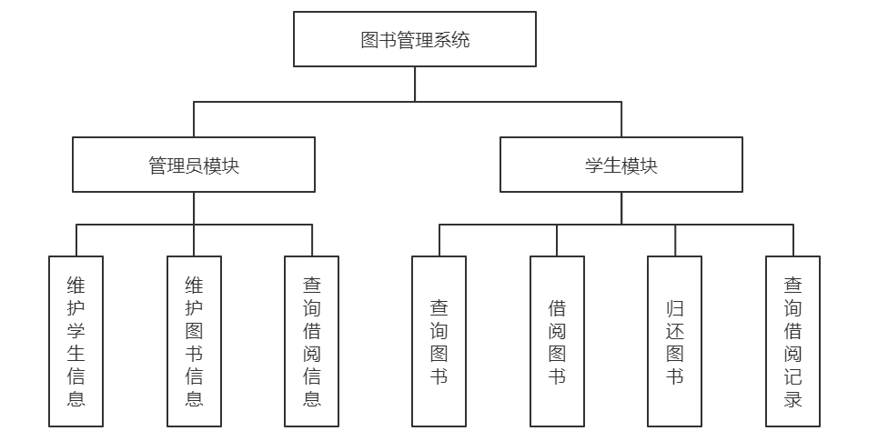
【图书馆管理系统的UML奥秘】:全面解码用例、活动、类和时序图(5图表精要)
# 摘要
本文探讨了统一建模语言(UML)在图书馆管理系统设计中的重要性,以及其在分析和设计阶段的核心作用。通过构建用例图、活动图和类图,本文揭示了UML如何帮助开发者准确捕捉系统需求、设计交互流程和定义系统结构。文中分析了用例图在识别主要参与者和用例中的应用,活动图在描述图书检索、借阅和归还流程中的作用,以及类图在定义图书类、读者类和管理员类之间的关系。
NVIDIA ORIN NX开发指南:嵌入式开发者的终极路线图

# 摘要
本文详细介绍了NVIDIA ORIN NX平台的基础开发设置、编程基础和高级应用主题。首先概述了该平台的核心功能,并提供了基础开发设置的详细指南,包括系统要求、开发工具链安装以及系统引导和启动流程。在编程基础方面,文章探讨了NVIDIA GPU架构、CUDA编程模型以及并行计算框架,并针对系统性能调优提供了实用
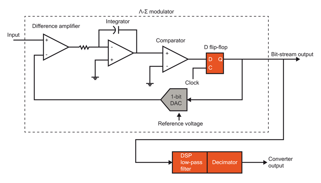
【Sigma-Delta ADC性能优化】:反馈与前馈滤波器设计的精髓
# 摘要
Sigma-Delta模数转换器(ADC)因其高分辨率和高信噪比(SNR)而广泛应用于数据采集和信号处理系统中。本文首先概述了Sigma-Delta ADC性能优化的重要性及其基本原理,随后重点分析了反馈和前馈滤波器的设计与优化,这两者在提高转换器性能方面发挥着关键作用。文中详细探讨了滤波器设计的理论基础、结构设计和性能优化策略,并对Sigma-Delta
【实战演练】:富士伺服驱动器报警代码全面解析与应对手册
# 摘要
本文详细介绍了富士伺服驱动器及其报警代码的基础知识、诊断流程和应对策略。首先概述了伺服驱动器的结构和功能,接着深入探讨了报警代码的分类、定义、产生原因以及解读方法。在诊断流程章节中,提出了有效的初步诊断步骤和深入分析方法,包括使用富士伺服软件和控制程序的技巧。文章还针对硬件故障、软件配置错误提出具体的处理方法,并讨论了维护与预防措施的重要性。最后,通过案例分析和实战演练,展示了报警分析与故障排除的实际应用,并总结了相关经验与
【单片微机系统设计蓝图】:从原理到实践的接口技术应用策略
# 摘要
单片微机系统作为一种集成度高、功能全面的微处理器系统,广泛应用于自动化控制、数据采集、嵌入式开发和物联网等多个领域。本文从单片微机系统的基本原理、核心理论到接口设计和实践应用进行了全面的介绍,并探讨了在现代化技术和工业需求推动下该系统的创新发展方向。通过分析单片微机的工作原理、指令集、接口技术以及控制系统和数据采集系统的设计原理,本文为相关领域工程师和研究人员提供了理论支持和
【Java内存管理秘籍】:掌握垃圾回收和性能优化的艺术
# 摘要
本文全面探讨了Java内存管理的核心概念、机制与优化技术。首先介绍了Java内存管理的基础知识,然后深入解析了垃圾回收机制的原理、不同垃圾回收器的特性及选择方法,并探讨了如何通过分析垃圾回收日志来优化性能。接下来,文中对内存泄漏的识别、监控工具的使用以及性能调优的案例进行了详细的阐述。此外,文章还探讨了内存模型、并发编程中的内存管理、JVM内存参数调优及高级诊断工具的应用。最
信号处理进阶:FFT在音频分析中的实战案例研究

# 摘要
本文综述了信号处理领域中的快速傅里叶变换(FFT)技术及其在音频信号分析中的应用。首先介绍了信号处理与FFT的基础知识,深入探讨了FFT的理论基础和实现方法,包括编程实现与性能优化。随后,分析了音频信号的特性、采样与量化,并着重阐述了FFT在音频频谱分析、去噪与增强等方面的应用。进一步,本文探讨了音频信号的进阶分析技术,如时间-频率分析和高
FCSB1224W000升级秘籍:无缝迁移至最新版本的必备攻略

# 摘要
本文综述了FCSB1224W000升级的全过程,涵盖从理论分析到实践执行,再到案例分析和未来展望。首先,文章介绍了升级前必须进行的准备工作,包括系统评估、理论路径选择和升级后的系统验证。其次,详细阐述了实际升级过程
资源上传下载、课程学习等过程中有任何疑问或建议,欢迎提出宝贵意见哦~我们会及时处理!
点击此处反馈


专栏目录
最低0.47元/天 解锁专栏
买1年送3月
百万级
高质量VIP文章无限畅学
千万级
优质资源任意下载
C知道
免费提问 ( 生成式Al产品 )