MATLAB Control Systems Simulation: Detailed Steps for Building Models and Testing
发布时间: 2024-09-15 00:33:31 阅读量: 9 订阅数: 18 
# Chapter 1: The Role of MATLAB in Control System Simulation
Analysis and design of control systems are core aspects of the engineering domain, involving numerous theoretical and practical aspects. MATLAB (Matrix Laboratory), as an efficient numerical computing and simulation software, has been widely applied in the field of control systems, particularly advantageous in simulation and analysis. MATLAB provides a suite of powerful toolboxes, especially the Control Systems Toolbox, offering engineers and researchers a comprehensive solution from system modeling, analysis, design, to simulation testing. With MATLAB, it is straightforward to achieve the mathematical modeling, dynamic analysis, parameter optimization, and final simulation testing of control systems, significantly enhancing the development efficiency and reliability of control systems. This chapter will outline the critical role and importance of MATLAB in control system simulation.
# Chapter 2: Setting Up MATLAB Simulation Environment
## 2.1 Installing and Configuring MATLAB Software
### 2.1.1 System Requirements and Installation Steps
The installation of MATLAB is crucial for ensuring efficient and accurate simulation operations. Before installation, it is essential to understand the basic system requirements, including operating system compatibility and minimum hardware configurations.
- **Operating System Compatibility**: MATLAB officially supports installation on Windows, Mac OS X, and Linux platforms. Ensure that the operating system version is compatible with the upcoming MATLAB version.
- **Minimum Hardware Requirements**: According to MATLAB's official recommendations, at least a dual-core processor is required, with a memory suggestion of 8GB or more, and the hard disk space will vary depending on the installed toolboxes and accessories.
After completing the above preparations, begin the installation process:
1. Visit the MathWorks official website to download the MATLAB installation package.
2. Launch the installer and follow the instructions of the installation wizard.
3. Enter the product serial number and user information.
4. Select the installation path and additional products (such as Simulink, toolboxes, etc.).
5. Adhere to the license agreement and initiate the installation.
6. After installation, restart the computer to ensure that all settings take effect.
### 2.1.2 Starting MATLAB Software and Overview of the Interface
After successful installation, the first time MATLAB is started, a clean and intuitive interface design will be seen. The main interface includes the following parts:
- **Command Window**: This is the main area where users input commands and view outputs.
- **Workspace**: Displays all currently open variables and files.
- **Path and Additional Path Settings**: Customize MATLAB's search path to facilitate the calling of functions and scripts.
- **Toolbar**: Provides icons for quick access to commonly used features.
- **Current Folder**: Shows and manages files in the current working directory.
These interface elements can help us better manage simulation projects.
## 2.2 MATLAB Simulation Toolboxes
### 2.2.1 Introduction to the Control Systems Toolbox
The Control Systems Toolbox is a MATLAB toolbox dedicated to the analysis and design of control systems, providing a multitude of functions and algorithms for solving control system modeling, simulation, analysis, and design problems. Features include:
- **System Representation**: Transfer functions, state-space models, zero-pole analysis, etc.
- **System Analysis**: Stability analysis, frequency response, root locus, etc.
- **System Design**: PID controller design, state feedback controller design, etc.
The toolbox simplifies and enhances the efficiency of analyzing and designing control systems within the MATLAB environment.
### 2.2.2 Common Toolbox Functions and Commands
To help users better utilize the Control Systems Toolbox, this section introduces some commonly used functions and commands:
- `tf`: Creates a transfer function model.
- `ss`: Creates a state-space model.
- `step`: Performs time response analysis of the system.
- `bode`: Draws the system's Bode diagram.
- `feedback`: Calculates system feedback connections.
For instance, to create a simple first-order system transfer function and draw its step response, the following code can be used:
```matlab
s = tf('s');
sys = 1/(s+1); % Creates a transfer function
step(sys); % Draws the step response
```
The above code block creates a simple first-order system transfer function and uses the `step` function to draw its step response diagram.
## 2.3 MATLAB's Simulink Environment
### 2.3.1 Simulink Interface and Basic Operations
Simulink is MATLAB's graphical simulation environment, providing an interactive drag-and-drop interface for designing and simulating dynamic systems. With Simulink, users can visually construct complex control system models.
The basic Simulink interface components are as follows:
- **Model Window**: This is the main area for building models, where users can add and configure modules by dragging and dropping.
- **Library Browser**: Contains various function modules, such as continuous, discrete, mathematical operations, etc.
- **Model Browser**: Used for browsing the model hierarchy and quickly accessing model components.
When starting Simulink, basic steps are:
1. Open the Simulink interface and create a new model file.
2. Select the required modules from the library browser and drag them into the model window.
3. Connect the modules and configure module parameters.
4. Run the model simulation and observe the results.
### 2.3.2 Simulink Library Browser and Module Libraries
The library browser is an essential tool for organizing and retrieving modules in Simulink. In Simulink, modules are organized into multiple libraries, each containing modules of a specific category. For example, the `Sinks` library includes modules for displaying simulation results, while the `Sources` library includes modules for simulating input signals.
Each module has a series of configurable parameters to adapt to different simulation needs. For instance, in the `Continuous` library's `Integrator` module, users can set initial conditions, limit values, and other parameters.
When using Simulink for simulation, first, open the required module library, then select and add modules to the model. The interface of the Simulink library browser is as follows:
; % Creates a transfer function model
```
### 3.1.2 Representation of State-Space Models
State-space models are represented by a set of linear differential equations describing the system's dynamic behavior. The state-space representation is typically in the form of: x'(t) = Ax(t) + Bu(t) and y(t) = Cx(t) + Du(t), where x is the state vector, u is the input vector, y is the output vector, and A, B, C, D are system matrices. In MATLAB, state-space models can be represented using the `ss` function.
```matlab
A = [-2, 3; -1, 0]; % System matrix A
B = [1, 0; 0, 1]; % Input matrix B
C = [0, 1; 1, 0]; % Output matrix C
D = [0, 0; 0, 0]; % Direct transmission matrix D
sys_ss = ss(A, B, C, D); % Creates a state-space model
```
In MATLAB, functions such as `step`, `impulse`, `bode`, etc., can be used to analyze the stability and response characteristics of transfer functions or state-space models.
## 3.2 Construction of Control System Models
### 3.2.1 Using Simulink to Construct Models
Simulink is an add-on product to MATLAB, providing a visual environment for simulating, analyzing, and designing various complex dynamic systems. Using Simulink allows for intuitive construction of control system models without the need for writing complex code.
#### Construction Steps:
1. Open Simulink and create a new model file.
2. Drag the required modules from the Simulink library into the model window, such as source (Source) modules, sink (Sink) modules, mathematical operation modules, etc.
3. Connect these modules, set their parameters, and complete the entire system construction.
### 3.2.2 Setting and Adjusting Model Parameters
Setting and adjusting parameters in the Simulink model is crucial, as it directly affects the simulation results.
#### Parameter Setting Steps:
1. Double-click the module to open its parameter settings window.
2. Enter or adjust the corresponding values, such as gain, time constants, etc.
3. Before running the simulation, you can set overall simulation parameters through the "Simulation" menu under "Model Configuration Parameters" in Simulink, including the simulation step size and duration.
After the Simulink model is constructed, the simulation can be started with the "Run" button. Data flow and signal processing in the model will proceed in order, ultimately yielding the system's dynamic response.
## 3.3 System Response and Stability Analysis
### 3.3.1 Simulation of System Time Response
The time response analysis of systems is an essential part of control system design, mainly evaluating the response characteristics of the system to specific inputs.
#### Simulation Steps:
***plete system model construction in Simulink.
2. Set simulation time and ensure all module parameters are configured.
3. Run the simulation and observe the output results. The output changes of the system can be visually observed through modules like the Oscilloscope (Scope).
### 3.3.2 System Frequency Response and Bode Diagram Analysis
Frequency response analysis helps to understand system behavior at different frequencies, and the Bode diagram is a commonly used tool to describe the system's amplitude-frequency and phase-frequency characteristics.
#### Analysis Steps:
1. Use MATLAB's `bode` function to directly calculate and draw the system's Bode diagram.
2. Or, in Simulink, add the Bode Plot module and run the simulation to observe the Bode diagram.
3. Analyze the slope, cutoff frequency, phase margin, and gain margin of the Bode diagram to evaluate the system's stability.
MATLAB and Simulink provide a powerful set of tools for constructing and analyzing control system models, making it more convenient and efficient for engineers to design and optimize.
```mermaid
flowchart LR
A[Establish Mathematical Model] --> B[Use tf Function to Represent Transfer Function]
A --> C[Use ss Function to Represent State-Space Model]
D[Build Simulink Model] --> E[Set Module Parameters]
F[Simulate Time Response] --> G[Observe Output Results]
H[Conduct Frequency Response Analysis] --> I[Draw Bode Diagram]
B --> D
C --> D
E --> F
G --> H
```
Through these steps and tools, in-depth understanding and efficient analysis of control systems can be achieved. As the complexity of the model increases, the advantages of using MATLAB and Simulink for model construction and analysis become more apparent.
# Chapter 4: Practical Application of Control System Simulation
## 4.1 Control System Simulation Testing
### 4.1.1 Designing Simulation Testing Schemes
Before conducting control system simulation testing, a detailed testing scheme must be designed first. The testing scheme should include a detailed description of the testing objectives, environment setup, testing steps, and expected results. Taking a simple proportional-integral-derivative (PID) controller as an example, we can design the following testing scheme:
#### Testing Objectives
Ensure that the PID controller can effectively compensate for system errors, achieving the desired stability and accuracy in the output response.
#### Testing Environment
- Use MATLAB/Simulink environment.
- Prepare a model of a linear controlled object.
- Design PID controller parameters, initially setting the values for proportional (P), integral (I), and derivative (D).
#### Testing Steps
1. Construct a Simulink model of the control system, including the controlled object and PID controller.
2. Set a step input signal as a reference for testing.
3. Run the simulation and record the output response data.
4. Adjust the PID parameters, repeat steps 2 and 3 until the optimal parameters are found.
5. Analyze the output response curve and verify the system's stability and accuracy.
#### Expected Results
- With different PID parameters, the system output should gradually approach the reference signal, showing the system's dynamic characteristics.
- A set of PID parameters should be found that minimizes the overshoot of the system response and shortens the adjustment time.
### 4.1.2 Analyzing Simulation Results and Optimizing Design
Analyzing simulation results is a critical part of simulation testing, requiring the comparison of response curves under different parameters to determine the optimal controller parameters. In MATLAB, we can utilize the data analysis tools provided by Simulink, such as oscilloscopes, spectrum analyzers, etc., to observe the system's dynamic response.
In the optimization design phase, we can use Simulink's automatic optimization feature or manually adjust the PID parameters. Automatic optimization features, such as Simulink Design Optimization, can help automatically adjust parameters to meet performance requirements. If manually adjusting parameters, adjust the P, I, and D values based on the system response curve and rerun the simulation.
```matlab
% Taking a simple PID controller as an example, set the PID parameters
Kp = 100; % Proportional gain
Ki = 50; % Integral gain
Kd = 10; % Derivative gain
% Use Simulink's PID Controller module to set parameters
set_param('pid_example/PID Controller', 'P', num2str(Kp), 'I', num2str(Ki), 'D', num2str(Kd));
```
In the above code, the `set_param` function is used to set parameters for a specific module in the Simulink model. The parameters `'P'`, `'I'`, and `'D'` correspond to the three parameters of the PID controller. When adjusting these parameters, it is necessary to carefully observe the system response and find the combination of parameters that optimizes performance.
## 4.2 System Fault Simulation and Diagnosis
### 4.2.1 Methods for Constructing Fault Models
In control system simulation, simulating system faults is a key step in evaluating the robustness of control algorithms. Constructing fault models usually requires an understanding of the actual system's fault modes, including sensor faults, actuator faults, line faults, etc. In MATLAB, fault models can be constructed in the following ways:
- **Modify system parameters**: Simulate actual faults by changing certain parameters in the system model. For example, a sensor fault can be simulated by increasing the resistance value.
- **Add signal interference**: Add noise or interference to the signal path to simulate sensor or actuator anomalies.
- **Use Simulink's fault modules**: Simulink provides some fault modules, such as the Actuator Failure module, which can be conveniently added to the model to simulate faults.
```matlab
% Simulate sensor faults, assuming a 5% offset needs to be added to the sensor output
add_block('simulink/Commonly Used Blocks/Step', 'sensor_fault_model/Offset');
set_param('sensor_fault_model/Offset', 'Time', '10', 'Amplitude', '0.05');
```
In the above code, we use the `add_block` and `set_param` functions to add a Step module to the Simulink model and set its parameters to simulate a sensor offset fault.
### 4.2.2 Fault Diagnosis and Fault-Tolerant Control
Fault diagnosis is the process by which a control system can promptly detect and identify the type and location of faults when they occur. Fault-tolerant control (FTC) ensures that the system can continue to operate as intended or safely reach the next checkpoint after a fault occurs.
In MATLAB, advanced control algorithms such as Model Predictive Control (MPC) and Adaptive Control can be used to achieve fault-tolerant control. At the same time, fault diagnosis algorithms such as Kalman filters, neural networks, rule-based diagnostic systems, etc., can be used to detect and diagnose faults.
```matlab
% A simplified example of using MPC for fault-tolerant control
mpcObj = mpc(CONTROL_SYSTEM); % CONTROL_SYSTEM is the system model to be controlled
mpcObj.Weights.ManipulatedVariablesRate = 0; % Reduce the rate of change in control actions, increasing system robustness
mpcObj.Weights.OutputVariables = 1; % Impose a heavy penalty on output variables to reduce errors
% Set the fault diagnosis logic for the model predictive controller
```
In practical applications, it is necessary to design appropriate fault-tolerant control logic based on the characteristics of the system and write code for fault diagnosis and handling.
## 4.3 Comparative Analysis of Real Systems and Simulations
### 4.3.1 Acquisition and Processing of Experimental Data
When comparing the simulation model and the real system, it is first necessary to ensure that experimental data is accurately obtained from the real system. The acquisition of data may require various sensors and appropriate data acquisition hardware devices. After obtaining the data, preprocessing is needed, such as filtering and noise reduction, data normalization, and removal of outliers.
```matlab
% Load data collected from the real system
load('real_system_data.mat');
% Use a filter to denoise the data
data_filtered = filtfilt(b, a, raw_data);
% Use the processed data for further analysis
```
In the above MATLAB code, the `load` function is used to load the data file. The `filtfilt` function is used for filtering, where `b` and `a` are filter coefficients, and `raw_data` is the original unprocessed data.
### 4.3.2 Analysis of Differences Between Simulation and Actual Systems
The simulation model is an approximate representation of the real system, but in practical applications, there will always be some differences. The purpose of comparative analysis is to identify these differences and further optimize the simulation model to better reflect the real-world situation. The differences may arise from various aspects, such as inaccurate model parameters, unconsidered dynamic factors, changes in the external environment, etc.
```matlab
% Compare the simulation results with the experimental data and calculate the differences
difference = abs(real_system_response - simulation_response);
% Analyze the differences, for example, by drawing a difference graph
figure;
plot(time_vector, difference);
title('Difference Analysis');
xlabel('Time');
ylabel('Difference Magnitude');
```
The above MATLAB code segment first calculates the difference between the real system's response and the simulation model output. Then, by drawing a difference graph, the degree of difference between the two is visually displayed. Through difference analysis, we can further adjust the simulation model to make it more precise.
The above content describes the practical application of control system simulation, including designing simulation testing schemes, analyzing simulation results, conducting system fault simulation and diagnosis, and performing a comparative analysis of real systems and simulations. Through these steps, engineers can ensure the accuracy and reliability of control algorithms before actually deploying control strategies.
# Chapter 5: Advanced Techniques in Control System Simulation
After discussing the basic applications of MATLAB in control system simulation, this chapter will delve into some advanced simulation techniques. These techniques are crucial for understanding and analyzing the dynamic behavior of complex control systems. This chapter will focus on parameter scanning and optimization techniques, nonlinear system simulation analysis, and the advanced applications of real-time simulation and hardware-in-the-loop testing.
## 5.1 Parameter Scanning and Optimization Techniques
### 5.1.1 Parameter Scanning Methods and Applications
In control system design and simulation, parameter scanning is a very important step. Through parameter scanning, designers can understand the impact of different parameter changes on system performance and find the best design parameters. MATLAB provides various parameter scanning methods, including but not limited to using loops, scripts, simulation parameter scanning tools in Simulink, and specialized optimization toolboxes.
A basic method for parameter scanning in MATLAB is to use a `for` loop, as shown in the example below:
```matlab
% Initialize parameter ranges
param_values = linspace(0, 10, 100); % For example, parameter range from 0 to 10
results = zeros(1, length(param_values)); % Initialize result storage array
for i = 1:length(param_values)
% Set parameters
param_to_scan = param_values(i);
% Here is simulation code, for example, updating Simulink model parameters
% run('model_name.slx', 'ParamName', num2str(param_to_scan));
% Here can be data acquisition after Simulink simulation
% results(i) = ... % Get simulation results
end
```
Parameter scanning can also be achieved through Simulink's simulation parameter scanning tool. Simulink allows users to use the "Simulation Parameter Scanning" interface to specify a series of parameter values and execute a simulation for each parameter value, collecting and analyzing results.
### 5.1.2 Selection and Implementation of Optimization Algorithms
After determining the impact of parameters on system performance, it is often necessary to find a set of optimal parameters to meet specific performance indicators. MATLAB provides various optimization algorithms, including genetic algorithms (`ga`), particle swarm optimization (`particleswarm`), etc., which can be used to solve parameter optimization problems.
A basic example of using the optimization toolbox in MATLAB is to use the `fmincon` function to find the optimal solution to a design problem, as shown in the example below:
```matlab
% Define the objective function
objective = @(x) (x(1) - 1)^2 + (x(2) - 2)^2;
% Define nonlinear constraints
nonlcon = @(x) deal([], [x(1)^2 + x(2)^2 - 10]);
% Define initial guess
x0 = [0.5, 0.5];
% Optimization options
options = optimoptions('fmincon', 'Algorithm', 'sqp');
% Execute optimization
[x_opt, fval] = fmincon(objective, x0, [], [], [], [], [], [], nonlcon, options);
% Output results
disp('Optimal solution:');
disp(x_opt);
disp('Objective function value:');
disp(fval);
```
In this example, the `fmincon` function is used to find the parameter values that minimize the objective function while satisfying the nonlinear constraints. The `options` variable allows users to choose different algorithms to optimize performance.
## 5.2 Nonlinear System Simulation Analysis
### 5.2.1 Characteristics and Modeling of Nonlinear Systems
Nonlinear systems are an advanced topic in the field of control system simulation. The characteristics of nonlinear systems are that the output is not a linear function of the input, making the analysis and control of nonlinear systems much more complex than linear systems. The behavior of nonlinear systems may include phenomena such as limit cycles, bifurcations, and chaos.
In MATLAB, the modeling of nonlinear systems usually involves writing or calling dynamic equations. A simple one-dimensional nonlinear system's dynamic model can be represented by a difference equation:
```matlab
% Initialize state and parameters
x = 1; % Initial state
param = 0.5; % System parameter
% Simulate multiple time steps
for t = 1:100
x = param * x * (1 - x); % Logistic map as an example
disp(['Time step:', num2str(t), ', State value:', num2str(x)]);
end
```
### 5.2.2 Advanced Techniques for Nonlinear System Simulation
For nonlinear system simulation, MATLAB provides several advanced analysis techniques. For example, analyzing the system's phase space diagram can provide an intuitive understanding of the system's dynamic behavior. A phase space diagram is a trajectory graph of the system's state variables over time.
```matlab
% Example of a phase space diagram in MATLAB
% Here, a simple two-dimensional nonlinear system is used as an example
x = linspace(0, 2*pi, 1000);
y = sin(x);
plot(x, y);
xlabel('State variable x');
ylabel('State variable y');
title('Phase space diagram of a nonlinear system');
grid on;
```
In addition, bifurcation diagrams are also an important tool for analyzing the behavior changes of nonlinear systems with parameter variations. There is no built-in function in MATLAB to directly generate bifurcation diagrams, but it can be achieved through programming.
## 5.3 Real-Time Simulation and Hardware-in-the-Loop Testing
### 5.3.1 Introduction to Real-Time Simulation Technology
Real-time simulation technology refers to the ability of the simulation system to operate under strict time constraints, simulating the real-time characteristics of actual system operation. Real-time simulation is particularly important for control systems, especially in situations where real-time control strategies need to be verified. MATLAB's real-time simulation toolbox (xPC Target) provides users with methods for real-time simulation.
Real-time simulation typically involves the following steps:
1. Design a real-time executable model.
2. Configure the real-time target.
3. Build a real-time application using the real-time application editor.
4. Run the real-time application on the target hardware.
### 5.3.2 Construction and Verification of Hardware-in-the-Loop Testing
Hardware-in-the-loop (HIL) testing is an effective method for verifying and testing real-time control systems. Through HIL testing, real hardware devices can be combined with a simulated environment for testing. In MATLAB, the Simulink Real-Time toolbox can be used to build an HIL testing environment.
The basic steps of HIL testing include:
1. Create a Simulink model containing real-time hardware interfaces.
2. Generate real-time code and download it to the target hardware.
3. Run real-time tests and monitor the hardware response.
4. Analyze test results and optimize.
### 5.3.3 Application Scenarios of Real-Time Simulation
Real-time simulation and HIL testing have extensive applications in the automotive, aerospace, robotics, and other fields. For example, in the automotive industry, HIL testing is used to verify the performance of automotive electronic control units (ECUs). By connecting ECUs to a virtualized vehicle powertrain, engineers can simulate vehicle dynamic behavior in a laboratory environment without actual vehicles.
Through these advanced simulation techniques, designers and engineers of control systems can more deeply understand the dynamic characteristics of the system and verify and test control strategies in a safe simulation environment. The proficient application of these techniques is crucial for ensuring the reliability and performance of modern control systems.
# Chapter 6: Case Studies in Control System Simulation
## 6.1 Motor Control System Simulation Case
### 6.1.1 Construction of Motor Control Systems
Motor control systems are an essential branch of electrical engineering, involving various aspects such as motor startup, acceleration, braking, and torque control. Within the MATLAB environment, Simulink can quickly build a simulation model of motor control systems, providing great convenience for design and testing.
For a basic DC motor control system, the following components generally need to be constructed:
- Motor model: Including parameters such as motor resistance, inductance, back-EMF coefficient, etc.
- Drive circuit: Depending on the control strategy, it can be a simple power amplifier circuit or a complex inverter circuit.
- Sensor: Used to detect motor feedback signals such as speed, position, or current.
- Controller: Such as PID controllers, state feedback controllers, etc., to implement control algorithms.
In Simulink, these parts can be constructed by directly dragging modules, connecting them according to the operational principle of the motor control system. For example, the motor model can be realized through the DC Motor module in Simulink, and the control algorithm can be accomplished through modules in the Simulink Control Systems Toolbox.
### 6.1.2 Analysis of Simulation Results and Applications
After completing the simulation, we usually focus on the following aspects of the results:
- The system's startup and acceleration performance, understanding the time and overshoot required for the motor to reach rated speed from a standstill.
- Steady-state performance, including the motor's speed stability under different load conditions.
- The controller's response characteristics, such as the rapidity, stability, and overshoot of step response.
- The system's resistance to external interference, such as performance during sudden load changes.
By analyzing these data, the motor control system can be evaluated and optimized. For example, if the step response has too much overshoot, it may be necessary to adjust the PID controller parameters; if the system's response to sudden load changes is slow, it may be necessary to add feedback links or use more advanced control strategies.
The following is a simplified code example showing how to set up a DC motor simulation in MATLAB:
```matlab
% First, create a Simulink model for the motor and controller
simulinkModel = 'DC_Motor_Simulation.slx';
open_system(simulinkModel);
% Simulate, setting the simulation time
set_param(simulinkModel, 'StopTime', '10');
sim(simulinkModel);
% Get simulation data and analyze
outputData = simout.Data;
figure; plot(outputData);
title('Motor Speed Response Curve');
xlabel('Time (s)');
ylabel('Speed (rpm)');
grid on;
```
In this simulation, we created a Simulink model named `DC_Motor_Simulation.slx` and set the simulation time. The `open_system` function opens the model, the `set_param` function configures the model properties, and the `sim` function runs the simulation. After the simulation, we use the `plot` function to display the motor's speed response curve.
## 6.2 Aerospace Control System Simulation Case
### 6.2.1 Overview of Aerospace Control Systems
The complexity of aerospace control systems lies in their need to ensure reliable operation under extreme environmental conditions, including high dynamics, uncertainty, strong nonlinearity, and parameter variations. Such systems typically need to have the following characteristics:
- High reliability and safety
- High-performance dynamic response and precise control
- Good robustness, able to operate stably under different environments and parameter variations
To achieve these goals, aerospace control systems often adopt advanced control strategies, such as adaptive control, robust control, model predictive control, etc.
### 6.2.2 Case Simulation and Performance Evaluation
Simulating aerospace control systems in the MATLAB/Simulink environment typically includes the following steps:
- Establish the dynamic model of the controlled object, such as the motion equations of an airplane or rocket.
- Implement the required control algorithms, such as a flight control system (FCS) or attitude control system (ACS).
- Set simulation scenarios to simulate different flight conditions and missions.
- Run the simulation and collect data, such as flight path, attitude angle, speed, and acceleration.
- Analyze the data to evaluate the performance of the control system, such as tracking accuracy, stability, response time, etc.
The following is a simple example code for loading an aerospace control system's Simulink model in MATLAB and performing simulation:
```matlab
% Load an aerospace control system's Simulink model
aeroSimulinkModel = 'Aerospace_Control_System.slx';
open_system(aeroSimulinkModel);
% Set simulation parameters, such as initial conditions for the flight mission
set_param(aeroSimulinkModel, 'InitialCondition', '[0; 0; 0; 0; 0; 0]');
% Run the simulation
set_param(aeroSimulinkModel, 'StopTime', '200');
sim(aeroSimulinkModel);
% Analyze simulation results
% Assuming the results are saved in the variable output
output = simout.Data;
% Further analysis code can be added according to specific needs
```
In this case, we loaded a Simulink model named `Aerospace_Control_System.slx` and set the initial conditions for the flight mission. After the simulation, we obtained the simulation data and can perform further performance evaluation.
## 6.3 Autonomous Vehicle Control Simulation Case
### 6.3.1 Introduction to Autonomous Vehicle Control Systems
Autonomous vehicle control systems are complex systems that integrate perception, decision-making, planning, and execution functions. It usually includes the following key parts:
- Perception system: Using various sensors such as radar, laser scanners (Lidar), cameras, etc., to obtain environmental information around the vehicle.
- Decision-making system: Based on perception data and map information, behavior decision-making and path planning are carried out.
- Execution system: Converts decisions into actual vehicle movements, including steering, acceleration, and braking control signals.
- Control system simulation: Simulates the entire vehicle operation process in a simulation environment to verify the effectiveness of control strategies.
MATLAB/Simulink provides a series of tools to support the simulation of autonomous vehicle control systems, such as the Autonomous Navigation Toolbox, which can help users build and test autonomous vehicle control systems.
### 6.3.2 Simulation Environment Setup and Testing Strategies
When setting up the simulation environment, factors to consider include:
- Simulating real-world road environments and traffic conditions.
- Designing reasonable test scenarios, such as vehicle following, overtaking, intersections, etc.
- Simulating various extreme weather and lighting conditions to test the system's performance under these conditions.
In MATLAB/Simulink, the following steps can be taken for simulation:
- Use third-party tools such as CarSim, PreScan, etc., integrated with MATLAB/Simulink to obtain more accurate vehicle dynamics models.
- Simulate the vehicle's sensors and actuators through Simulink models.
- Design test plans in MATLAB scripts and run simulations to collect data.
- Use MATLAB for data analysis to evaluate the effectiveness and safety of control strategies.
The following is a simplified MATLAB script example for setting up the simulation environment for autonomous vehicle control systems:
```matlab
% Start the simulation environment and vehicle model
carModel = 'Autonomous_Vehicle.slx';
open_system(carModel);
% Set simulation parameters, such as weather conditions and road types
weather = 'clear';
roadType = 'urban';
% Run the simulation
set_param(carModel, 'Weather', weather, 'RoadType', roadType);
sim(carModel);
% Collect simulation data
% Assuming vehicle state data is saved in the variable vehicleState
vehicleState = simout.Data;
% Analyze vehicle state data to evaluate the performance of the control system
% Further analysis code can be added according to specific needs
```
In this example, we loaded a Simulink model named `Autonomous_Vehicle.slx` and ran the simulation based on different weather conditions and road types. After the simulation, we collected vehicle state data for analysis.
Through the detailed elaboration of the above chapters, we can see the significant role of MATLAB/Simulink as a simulation tool in control system simulation. Through specific case studies, we can more deeply understand its value and potential in practical applications. For control system designers, mastering these simulation techniques is key to improving work efficiency and system performance.
 最低0.47元/天 解锁专栏
 送3个月
 百万级
高质量VIP文章无限畅学
百万级
高质量VIP文章无限畅学
 千万级
优质资源任意下载
千万级
优质资源任意下载
 C知道
免费提问 ( 生成式Al产品 )
C知道
免费提问 ( 生成式Al产品 )
0
0
相关推荐

专栏目录
最低0.47元/天 解锁专栏
送3个月
百万级
高质量VIP文章无限畅学
千万级
优质资源任意下载
C知道
免费提问 ( 生成式Al产品 )
最新推荐
Python list remove与列表推导式的内存管理:避免内存泄漏的有效策略
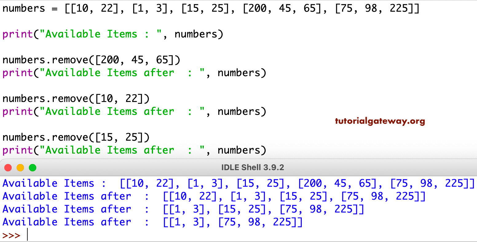
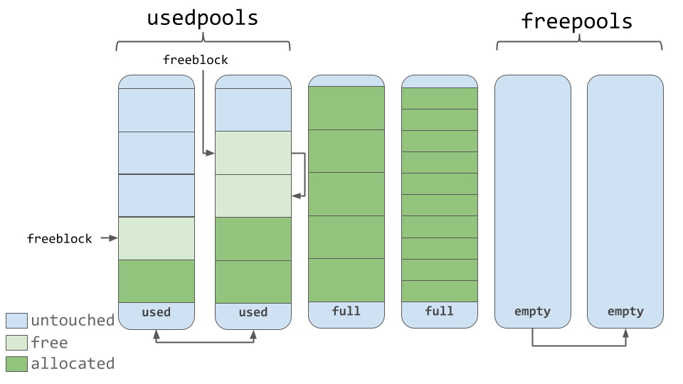
# 1. Python列表基础与内存管理概述
Python作为一门高级编程语言,在内存管理方面提供了众多便捷特性,尤其在处理列表数据结构时,它允许我们以极其简洁的方式进行内存分配与操作。列表是Python中一种基础的数据类型,它是一个可变的、有序的元素集。Python使用动态内存分配来管理列表,这意味着列表的大小可以在运行时根据需要进
Python装饰模式实现:类设计中的可插拔功能扩展指南
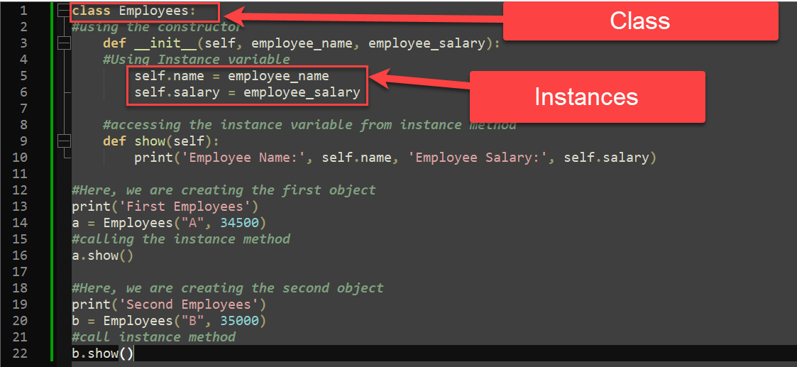
# 1. Python装饰模式概述
装饰模式(Decorator Pattern)是一种结构型设计模式,它允许动态地添加或修改对象的行为。在Python中,由于其灵活性和动态语言特性,装饰模式得到了广泛的应用。装饰模式通过使用“装饰者”(Decorator)来包裹真实的对象,以此来为原始对象添加新的功能或改变其行为,而不需要修改原始对象的代码。本章将简要介绍Python中装饰模式的概念及其重要性,为理解后
Python函数性能优化:时间与空间复杂度权衡,专家级代码调优
# 1. Python函数性能优化概述
Python是一种解释型的高级编程语言,以其简洁的语法和强大的标准库而闻名。然而,随着应用场景的复杂度增加,性能优化成为了软件开发中的一个重要环节。函数是Python程序的基本执行单元,因此,函数性能优化是提高整体代码运行效率的关键。
## 1.1 为什么要优化Python函数
在大多数情况下,Python的直观和易用性足以满足日常开发
【Python项目管理工具大全】:使用Pipenv和Poetry优化依赖管理

# 1. Python依赖管理的挑战与需求
Python作为一门广泛使用的编程语言,其包管理的便捷性一直是吸引开发者的亮点之一。然而,在依赖管理方面,开发者们面临着各种挑战:从包版本冲突到环境配置复杂性,再到生产环境的精确复现问题。随着项目的增长,这些挑战更是凸显。为了解决这些问题,需求便应运而生——需要一种能够解决版本
【递归与迭代决策指南】:如何在Python中选择正确的循环类型
# 1. 递归与迭代概念解析
## 1.1 基本定义与区别
递归和迭代是算法设计中常见的两种方法,用于解决可以分解为更小、更相似问题的计算任务。**递归**是一种自引用的方法,通过函数调用自身来解决问题,它将问题简化为规模更小的子问题。而**迭代**则是通过重复应用一系列操作来达到解决问题的目的,通常使用循环结构实现。
## 1.2 应用场景
递归算法在需要进行多级逻辑处理时特别有用,例如树的遍历和分治算法。迭代则在数据集合的处理中更为常见,如排序算法和简单的计数任务。理解这两种方法的区别对于选择最合适的算法至关重要,尤其是在关注性能和资源消耗时。
## 1.3 逻辑结构对比
递归
Python数组在科学计算中的高级技巧:专家分享

# 1. Python数组基础及其在科学计算中的角色
数据是科学研究和工程应用中的核心要素,而数组作为处理大量数据的主要工具,在Python科学计算中占据着举足轻重的地位。在本章中,我们将从Python基础出发,逐步介绍数组的概念、类型,以及在科学计算中扮演的重要角色。
## 1.1 Python数组的基本概念
数组是同类型元素的有序集合,相较于Python的列表,数组在内存中连续存储,允
Python列表与数据库:列表在数据库操作中的10大应用场景

# 1. Python列表与数据库的交互基础
在当今的数据驱动的应用程序开发中,Python语言凭借其简洁性和强大的库支持,成为处理数据的首选工具之一。数据库作为数据存储的核心,其与Python列表的交互是构建高效数据处理流程的关键。本章我们将从基础开始,深入探讨Python列表与数据库如何协同工作,以及它们交互的基本原理。
## 1.1
字典索引在Python中的高级用法与性能考量

# 1. Python字典索引基础
在Python中,字典是一种核心数据结构,提供了灵活且高效的索引功能。本章将介绍字典的基本概念以及如何使用索引来操作字典。
索引与数据结构选择:如何根据需求选择最佳的Python数据结构
# 1. Python数据结构概述
Python是一种广泛使用的高级编程语言,以其简洁的语法和强大的数据处理能力著称。在进行数据处理、算法设计和软件开发之前,了解Python的核心数据结构是非常必要的。本章将对Python中的数据结构进行一个概览式的介绍,包括基本数据类型、集合类型以及一些高级数据结构。读者通过本章的学习,能够掌握Python数据结构的基本概念,并为进一步深入学习奠
【Python字典的并发控制】:确保数据一致性的锁机制,专家级别的并发解决方案

# 1. Python字典并发控制基础
在本章节中,我们将探索Python字典并发控制的基础知识,这是在多线程环境中处理共享数据时必须掌握的重要概念。我们将从了解为什么需要并发控制开始,然后逐步深入到Python字典操作的线程安全问题,最后介绍一些基本的并发控制机制。
## 1.1 并发控制的重要性
在多线程程序设计中
资源上传下载、课程学习等过程中有任何疑问或建议,欢迎提出宝贵意见哦~我们会及时处理!
点击此处反馈


专栏目录
最低0.47元/天 解锁专栏
送3个月
百万级
高质量VIP文章无限畅学
千万级
优质资源任意下载
C知道
免费提问 ( 生成式Al产品 )