Master MATLAB Control Systems from Scratch: Full Process Analysis and Practical Exercises
发布时间: 2024-09-15 00:30:26 阅读量: 37 订阅数: 40 

MNIST CNN from scratch:CNN 对从头开始编码的数字进行分类-matlab开发
# 1. Introduction to MATLAB Control Systems
In the modern industrial and technological fields, MATLAB, as an important mathematical computation and simulation tool, is widely and deeply applied in the design and analysis of control systems. This chapter aims to offer a crash course for beginners to familiarize themselves with the basic operations of MATLAB and the fundamental process of designing control systems. We will first briefly introduce the functionalities of MATLAB software and its installation method, then outline the primary applications of MATLAB in control system analysis. Additionally, this chapter will provide some foundational knowledge of control theory and a preliminary introduction to related MATLAB commands, laying a solid foundation for further in-depth study. Whether you are a beginner in the field of automatic control or a reader with some knowledge of MATLAB looking to enhance your control theory application skills, this chapter will serve as an excellent starting point.
# 2. Basic MATLAB Theory and Operations
### 2.1 MATLAB Basic Syntax
As an advanced programming language used for numerical computation, data analysis, and visualization, MATLAB's basic syntax is crucial. Mastering these foundational syntaxes is essential for performing complex tasks with MATLAB.
#### 2.1.1 Variables, Matrix, and Array Operations
In MATLAB, variables do not require explicit declaration of their data types, making programming more flexible. The most commonly used structures are matrices and arrays, which are the basis for mathematical operations.
```matlab
% Defining a matrix
A = [1 2; 3 4];
% Defining an array
B = [5, 6, 7];
% Matrix multiplication
C = A * B;
% Matrix transpose
D = A';
```
In the above code, matrix `A` is defined by rows and columns. In MATLAB, matrix operations are vectorized, meaning they are automatically applied to each element. For instance, multiplying by 2 will affect every element of array `B`. Matrix `C` is obtained from the product of matrix `A` and array `B`, while `D` is the transpose of matrix `A`. All these operations involve basic mathematical computations, which are the cornerstone of building more complex systems and algorithms.
#### 2.1.2 Graphical Plotting and Data Visualization
MATLAB provides an abundance of functions for graphical plotting and data visualization, which are essential for understanding the results of data analysis and the behavior of control systems.
```matlab
% Generating data
x = 0:0.1:10;
y = sin(x);
% Plotting the graph
figure;
plot(x, y);
title('Sine Wave');
xlabel('Time');
ylabel('Amplitude');
grid on;
```
In the code above, we first create two variables `x` and `y`, representing time and amplitude, respectively. By calling the `plot` function, we draw them on a graph and add a title and axis labels using the `title`, `xlabel`, `ylabel` functions. The `grid on` command adds gridlines, facilitating the localization of data points.
### 2.2 Mathematical Foundations of MATLAB Control Systems
MATLAB plays a significant role in the analysis and design of control systems, mainly due to its powerful capabilities in mathematical computations, particularly in linear algebra and calculus.
#### 2.2.1 Applications of Linear Algebra in Control Systems
Linear algebra is an important tool in control engineering, involving matrix operations, eigenvalues, and eigenvectors, all of which are fundamental to control system analysis.
```matlab
% Creating a matrix
M = [2, -1, 0; -1, 2, -1; 0, -1, 1];
% Calculating eigenvalues and eigenvectors
[eigenvectors, eigenvalues] = eig(M);
% Displaying eigenvalues and corresponding eigenvectors
disp('Eigenvalues:');
disp(diag(eigenvalues));
disp('Corresponding eigenvectors:');
disp(eigenvectors);
```
In this code snippet, we define a matrix `M` first. Next, we use the `eig` function to compute the eigenvalues and eigenvectors of the matrix and store the results in the `eigenvalues` and `eigenvectors` variables. The `disp` function is used to display the results in the command window. The calculation of eigenvalues and eigenvectors is crucial for determining the stability and dynamic characteristics of a system.
#### 2.2.2 Calculus and Dynamic Analysis of Control Systems
Calculus is another fundamental mathematical tool in control theory, playing a key role in the analysis of system dynamic characteristics.
```matlab
% Defining time variable
t = 0:0.01:10;
% Defining the system's transfer function
num = [1]; % Numerator polynomial coefficients
den = [1, 3, 2]; % Denominator polynomial coefficients
sys = tf(num, den); % Creating transfer function model
% Plotting the unit step response
figure;
step(sys, t);
title('Unit Step Response');
xlabel('Time');
ylabel('Response');
```
In this code, we define the time variable `t`, create a transfer function `sys`, and use the `step` function to plot the unit step response of the system. Such dynamic analysis is essential for understanding and predicting the behavior of control systems over time.
The above sections demonstrate the powerful capabilities of MATLAB in basic theory and operations. It offers robust mathematical computation and data visualization through simple and intuitive syntax, making it an indispensable tool for control system analysis and design. As we delve into subsequent chapters, we will further explore how to leverage MATLAB to solve more complex control problems.
# 3. Control System Modeling and Simulation
## 3.1 Mathematical Modeling of Control Systems
In engineering practice and theoretical research, the design and analysis of control systems first require the establishment of accurate mathematical models, which is the basis for system simulation and control strategy design. The mathematical modeling of control systems mainly includes state-space representation and transfer function models and their conversions.
### 3.1.1 State-Space Representation
State-space representation describes the dynamic behavior of a system through a set of differential equations, with its core being the definition of the system's state variables. The choice of state variables directly affects the accuracy and complexity of the model.
```mermaid
flowchart LR
A[Define system state variables] --> B[Establish state equations]
B --> C[Determine output equations]
C --> D[State-space model]
```
Specifically, a typical linear time-invariant (LTI) system's state-space model can be represented as:
```mathematica
\begin{aligned}
& \dot{x}(t) = Ax(t) + Bu(t) \\
& y(t) = Cx(t) + Du(t)
\end{aligned}
```
Where \(x(t)\) is the state vector, \(u(t)\) is the input vector, \(y(t)\) is the output vector, and \(A\), \(B\), \(C\), and \(D\) are system matrices representing the evolution of the system state, the effect of input on the state, the effect of state on output, and the direct effect of input on output, respectively.
### 3.1.2 Transfer Function Models and Their Conversions
Transfer function models are another commonly used mathematical model in control system analysis, expressing the relationship between the system's input and output in the form of Laplace transforms. For LTI systems, the transfer function can be obtained by applying the Laplace transform to both sides of the state-space model equations.
```mermaid
graph LR
A[State-space model] --> |Laplace Transform| B[Transfer function model]
B --> C[Solve system characteristics]
C --> D[Frequency response analysis]
```
Transfer functions are typically represented as:
```mathematica
G(s) = \frac{Y(s)}{U(s)} = \frac{C(sI-A)^{-1}B + D}{sI-A}
```
Where \(Y(s)\) and \(U(s)\) are the Laplace transforms of the output and input, respectively. Transfer function models facilitate frequency and stability analyses of the system.
## 3.2 MATLAB's Application in System Simulation
MATLAB provides a powerful simulation tool called Simulink, capable of modeling the dynamic behavior of control systems, evaluating the feasibility of designs, and optimizing them.
### 3.2.1 Introduction to the Simulink Environment
Simulink is an add-on product to MATLAB, offering a visual design environment where users can build system models using drag-and-drop functionality. Simulink supports a variety of modules, including linear system modules, nonlinear modules, signal source, and signal receiver modules.
Steps to create a Simulink model typically include:
- Open Simulink and create a new model.
- Add and configure system components as needed.
- Connect the components to form a complete system.
- Set simulation parameters, such as simulation time and step size.
- Run the simulation and observe the results.
### 3.2.2 Case Study of System Simulation
Next, we will illustrate MATLAB's application in system simulation through a simple inverted pendulum control system simulation case.
#### Introduction to the Inverted Pendulum System
The inverted pendulum is a classic control problem aiming to design a controller that can stabilize the pendulum rod from a downward position to a vertical position within a finite time. The system can be abstracted as a second-order system with two state variables: position and angle.
#### Building the Simulink Model
```matlab
% Here provides the key code segment for building the inverted pendulum Simulink model
simulinkModel = 'pendulumSimulinkModel';
open_system(simulinkModel);
```
In Simulink, we need to build a dynamic model that includes the pendulum and wheel, add a control input, and sensors to measure the position and velocity of the pendulum. After model construction, we can perform simulation tests.
```matlab
% Simulation command
set_param(simulinkModel, 'StopTime', '5');
set_param(simulinkModel, 'SolverOptions', 'AutoInitiatorOn');
set_param(simulinkModel, 'SolverName', 'ode45');
simOut = sim(simulinkModel);
```
#### Result Analysis
After simulation, by plotting the curve of the pendulum position over time, we can visually observe the effectiveness of the control strategy and据此进行控制器的调整和优化。
```matlab
% Plotting the simulation results
figure;
plot(simOut.tout, simOut.yout);
xlabel('Time (s)');
ylabel('Pendulum Position');
title('Pendulum Position Over Time');
```
This chapter has detailedly explored the basic methods of control system mathematical modeling and MATLAB's specific applications in system simulation. Through the above content, readers should be able to understand and implement simple control system model construction and simulation analysis. The subsequent chapters will delve into the details of control strategy design and MATLAB's applications in control strategy optimization.
# 4. MATLAB Control Strategy Design
## 4.1 Stability Analysis of Control Systems
### 4.1.1 Pole Placement and Stability Criteria
In the design of control systems, pole placement is a key technique to ensure system stability. In the MATLAB environment, engineers can determine the position of system poles by calculating the roots of the system's characteristic equation. The key to system stability is that all poles must be located in the left half of the complex plane.
MATLAB provides the `roots` function to find the roots of polynomial equations and the `pole` function to directly calculate the system poles. For example, given a continuous-time linear system's transfer function `G(s) = 1/(s^2 + 4s + 3)`, we can calculate its poles using the following code:
```matlab
num = [1]; % Numerator polynomial coefficients
den = [1 4 3]; % Denominator polynomial coefficients
sys = tf(num, den); % Create transfer function model
poles = pole(sys); % Calculate and display the system poles
```
The stability criterion of pole placement states that if the real parts of all system poles are less than zero, then the system is stable. MATLAB can perform this process automatically or through manual programming. When writing code, it is important to note that the order of polynomial coefficients in MATLAB is arranged in descending order.
### 4.1.2 Routh-Hurwitz Stability Criterion
The Routh-Hurwitz stability criterion is another method for determining the stability of linear systems. This criterion constructs a Routh table to determine if all roots of the system characteristic equation are located in the left half of the complex plane.
Below is an example of constructing a Routh table using MATLAB:
```matlab
s = tf('s');
num = [1]; % Numerator polynomial coefficients
den = [1 4 3]; % Denominator polynomial coefficients
sys = num/den;
r = routh(sys); % Calculate the Routh table
```
After constructing the Routh table, the distribution of system poles can be analyzed by examining the first column. If there are no elements that change from positive to negative (or vice versa) in the first column, then the system is stable.
## 4.2 Control Design Methods
### 4.2.1 PID Controller Design and Debugging
The Proportional-Integral-Derivative (PID) controller is one of the most widely used controllers in control systems. The PID controller adjusts the output through three main parameters (proportional gain Kp, integral gain Ki, and derivative gain Kd) to achieve rapid and accurate tracking of the setpoint.
MATLAB provides design and analysis tools for PID controllers. Below is a simple example of PID design:
```matlab
Kp = 1;
Ki = 0.1;
Kd = 0.05;
controller = pid(Kp, Ki, Kd); % Create PID controller object
% Set target value and feedback value for simulation
setpoint = 10;
feedback = 0:0.05:10;
% Calculate control input through the PID controller
control_input = lsim(controller, feedback, setpoint);
% Plot response curve
figure;
plot(feedback, control_input);
title('PID Controller Response');
xlabel('Time');
ylabel('Control Input');
```
When designing a PID controller, engineers need to optimize controller performance by adjusting these three parameters: Kp, Ki, and Kd. MATLAB's `pidtune` function can automatically tune PID parameters.
### 4.2.2 State Feedback and Observer Design
State feedback control is a control strategy based on the system's internal states that can enhance system performance and stability. A state observer allows engineers to estimate system states indirectly without directly measuring all states.
MATLAB provides the `place` and `acker` functions to determine the state-space representation of a state feedback controller. Meanwhile, MATLAB's built-in observer design tool can assist engineers in designing a suitable observer. Below is an example of designing a state feedback controller and observer:
```matlab
% Given system state space representation
A = [0 1; -3 -4];
B = [0; 1];
C = [1 0];
D = 0;
sys = ss(A, B, C, D);
% Set the desired pole locations
desired_poles = [-1 -2];
% Design controller using state feedback
K = place(A, B, desired_poles);
% Design state observer
L = place(A', C', desired_poles)';
% Create closed-loop and observer systems
controller_sys = ss(A-B*K, B, eye(size(A)), zeros(size(B)));
observer_sys = ss(A-L*C, L, eye(size(A)), zeros(size(A)));
% Plot poles of closed-loop and observer systems
figure;
plot(tf(sys), 'b--');
hold on;
plot(tf(controller_sys), 'r');
plot(tf(observer_sys), 'g');
legend('Original System', 'Closed-loop System', 'Observer System');
title('State Feedback and State Observer Design');
```
When designing state feedback controllers and observers, it is crucial to choose the system matrix `A` and control matrix `B`, as well as the desired pole locations `desired_poles`. MATLAB's `place` function can find the state feedback gain matrix and observer gain matrix that meet specific performance requirements.
# 5. Advanced Applications of MATLAB in Control Systems
As we delve deeper into the design and analysis of control systems, MATLAB's applications extend beyond basic modeling and simulation. In this chapter, we will explore MATLAB's advanced applications in control systems, including optimizing control strategies and integrating with different tools. These advanced applications can help engineers develop more complex and efficient control solutions, improve system performance, and shorten development cycles.
## 5.1 Optimizing Control Strategies
The optimization of control systems is an eternal topic, with engineers constantly seeking more efficient control strategies to meet increasing performance demands. MATLAB offers powerful tools and function libraries for designing more robust and adaptable control systems.
### 5.1.1 Robust Control Design
Robust control design focuses on ensuring the stability of control systems when faced with model uncertainties or external disturbances. MATLAB's `robust` controller design toolbox provides strong support for designing such control systems. With this toolbox, designers can create robust control systems resistant to these uncertainties.
Designing robust controllers in MATLAB typically involves the following steps:
- Determine the system model, considering its uncertainties.
- Design a robust controller that meets the system's stability and performance requirements.
- Use functions from the `robust` toolbox to adjust and optimize controller parameters.
- Analyze the system's performance under different operating conditions to verify robustness.
A typical code example for designing a robust controller in MATLAB is as follows:
```matlab
% Define system model with uncertainty factors
P = ureal('P', 1, 'Percentage', 10); % Assume a 10% model error
G = tf(1, [1, 10, P]);
% Design an H∞ robust controller
K = hinfstruct('Controller', G);
% Analyze the performance of the closed-loop system
CL = feedback(K*G, 1);
step(CL);
```
### 5.1.2 Adaptive Control and Model Predictive Control
Adaptive control and model predictive control (MPC) are two advanced control strategies that allow the control system to automatically adjust its control strategy during operation based on changes in the environment.
Adaptive control is mainly suitable for systems with unknown or time-varying parameters. MATLAB provides a series of functions and methods for designing and implementing adaptive controllers through its adaptive control toolbox.
Model predictive control (MPC) is a model-based control strategy that solves an online optimization problem in each control cycle, predicting future system behavior and calculating the optimal control action for the current moment. MATLAB's model predictive control toolbox provides functions necessary for designing MPC controllers, such as:
```matlab
% Define predictive model
A = [1, 1; 0, 1];
B = [0.5; 1];
C = eye(2);
D = zeros(2, 1);
sys = ss(A, B, C, D);
% Design MPC controller
mpcController = mpc(sys, 1);
% Set optimization constraints and objectives
mpcController.Weights.OutputVariables = 0.1;
mpcController.Weights.ManipulatedVariablesRate = 0.01;
mpcController.MV = struct('Min',-10,'Max',10);
% Simulate MPC controller behavior
mpcSim = mpcsim(mpcController);
```
Through these advanced control strategies, engineers can design more intelligent and automated control systems to adapt to complex and ever-changing application environments.
## 5.2 Integration of MATLAB with Other Tools
MATLAB is not just a standalone tool; it can also integrate with other software and hardware to form a comprehensive solution. By collaborating with third-party tools, users can achieve data exchange, functional extension, and deep integration of applications.
### 5.2.1 MATLAB and Hardware Interfaces
MATLAB's ability to interface with hardware expands its applications in real control systems. For example, MATLAB can directly communicate with microcontrollers and single-board computers such as Arduino and Raspberry Pi for data acquisition, signal processing, and sending control commands.
In MATLAB, hardware communication can be achieved using supported hardware packages (e.g., Arduino Support Package). For example, the following code demonstrates how to control an LED on an Arduino board using MATLAB:
```matlab
% Initialize Arduino object
a = arduino('COM3');
% Create LED object
led = digitalpin(a, 13, 'output');
% Control LED
write(led, 1); % Turn on the LED
pause(2); % Wait for 2 seconds
write(led, 0); % Turn off the LED
```
### 5.2.2 MATLAB and Collaboration with Professional Software
In the development and testing of control systems, it is often necessary to work collaboratively with various professional software, such as CAD (Computer-Aided Design) software and PLC (Programmable Logic Controller) programming software. MATLAB's flexibility allows it to exchange data with these software and complement each other's functions.
For instance, MATLAB can import geometric model data from CAD software for mechanical dynamics simulation. Meanwhile, MATLAB code can be embedded into PLC programs to perform complex control algorithm calculations.
Below is a simple example showing how MATLAB can import geometric data from a CAD file for subsequent analysis:
```matlab
% Use MATLAB's CAD interface function
cadData = importGeometry('exampleCADfile.dxf');
% Check the characteristics of the geometric body
volume = volume(cadData);
disp(['The volume of the imported geometry is: ', num2str(volume)]);
```
Through integration with these professional software, engineers can fully utilize the advantages of various tools to achieve more precise and efficient development of control systems.
As technology continues to advance, MATLAB's applications in the field of control systems are constantly expanding. By mastering MATLAB's advanced functions and integration with other tools, engineers can design more complex and advanced control systems to meet the rapidly changing technological challenges of today's world. In Chapter 6, we will delve into practical application cases to explore MATLAB's actual use in industries and aerospace and other fields.
# 6. Practical Exercise: MATLAB's Application in Real Control Systems
## 6.1 Analysis of Actual Engineering Cases
### 6.1.1 Industrial Process Control System Case
Industrial process control systems are key technologies that ensure production processes are stable, efficient, and safe. Due to its powerful numerical computation capabilities and a wealth of toolboxes, MATLAB is widely used in the field of industrial automation. We take a typical chemical reaction process control as an example to demonstrate how MATLAB can play a unique role in real control systems.
**Step 1: Model Establishment and Simulation**
First, based on the principles of chemical reaction kinetics, establish the mathematical model of the chemical reaction process. In MATLAB, the symbolic computation toolbox can be used to derive the system's differential equation model. Then, using MATLAB's built-in numerical integration methods, such as `ode45`, perform numerical simulations on the model and use the `plot` function for result visualization.
```matlab
% Define symbolic variables and model equations
syms T(t) C(t) % T and C represent temperature and concentration, respectively
% Assume the differential equations are dT/dt = f(T,C) and dC/dt = g(T,C)
% ...
% Use MATLAB numerical solvers to solve differential equations
[T, C] = ode45(@(t, y) [f(t,y(1),y(2)); g(t,y(1),y(2))], [0, t_final], [T0, C0]);
% Plot simulation results
plot(T, C);
title('Chemical Reaction Process Simulation');
xlabel('Time');
ylabel('Variables');
```
**Step 2: Control System Design**
Next, design a temperature control system to maintain the temperature of the chemical reaction process. This typically involves adjusting controller parameters, such as those of a PID controller. The PID controller toolbox in MATLAB can be used for design, and simulation can be used to verify the control effect.
```matlab
% Design PID controller
Kp = 1; Ki = 1; Kd = 1;
controller = pid(Kp, Ki, Kd);
% Simulate temperature control system
% ...
```
### 6.1.2 Challenges in Aerospace Control Systems
In the aerospace field, the complexity of control systems and the high demand for reliability mean that design and testing must be rigorous. MATLAB offers a suite of tools, including Simulink, for modeling, simulation, and control of spacecraft.
**Case Study**
Taking a simplified satellite attitude control problem as an example, we explore how MATLAB can assist in designing and implementing an efficient control strategy. The Simulink model can simulate the physical dynamics of a satellite, including its motion in orbit and external disturbances.
**Implementation Steps**
1. Create a dynamic model of the satellite, including mass and inertia matrices.
2. Design an attitude control algorithm, such as PID control or more advanced control strategies.
3. Implement the control algorithm in Simulink and perform closed-loop simulation.
4. Analyze the simulation results and adjust controller parameters to optimize performance.
## 6.2 Project Practical Guidance
### 6.2.1 Steps from Theory to Practice
Learning how to apply MATLAB tools to the design and analysis of actual control systems is crucial in the transition from theory to practice. Below is a systematic set of steps to help readers turn their learned knowledge into practical skills.
1. **Understand Control System Requirements**: First, thoroughly understand the requirements and goals of the control system.
2. **Establish Mathematical Models**: Based on physical principles or experimental data, establish the mathematical model of the system.
3. **Choose Appropriate Control Strategies**: Based on the complexity of the model and control objectives, choose an appropriate control strategy.
4. **Simulation and Analysis**: Use MATLAB's Simulink or other tools for system simulation and analyze the results.
5. **Adjust and Optimize**: Adjust system parameters based on simulation results to optimize control performance.
6. **Hardware Implementation**: Deploy the control strategy on a hardware platform for actual testing.
### 6.2.2 System Design Report Writing and Project Management
Writing a detailed design report and effectively managing a project is key to success when implementing control system projects. Here are suggestions for writing system design reports and project management.
**Design Report Writing**
The design report should include:
- Introduction: Overview of the project background, goals, and main conclusions.
- System Design: Detailedly describe each stage of system design and the methods used.
- Control Strategy: Explain the reasons for choosing the control strategy and its advantages and disadvantages.
- Simulation and Analysis: Provide simulation results and analyze them.
- Experimental Results: If there is hardware implementation, include experimental data and result analysis.
- Conclusion and Recommendations: Summarize the entire project and provide suggestions for subsequent work.
**Project Management**
Effective project management includes the following aspects:
- Time Planning: Develop a detailed schedule and reasonably allocate the workload for each stage.
- Resource Management: Ensure that the necessary human, material, and financial resources for the project are rationally allocated and utilized.
- Risk Assessment: Identify potential risks in the project and develop countermeasures.
- Quality Control: Ensure that each stage of the project meets the predetermined quality standards.
- Communication Coordination: Regularly communicate with the project team and stakeholders to ensure information transparency and goal alignment.
Through the detailed introductions and case analyses in the above chapters, one can gain a comprehensive understanding of MATLAB's various applications in real control systems. From mathematical modeling, system simulation, to control strategy design, MATLAB provides a one-stop solution, significantly reducing the difficulty and cost of developing control systems.

 百万级
高质量VIP文章无限畅学
百万级
高质量VIP文章无限畅学
 千万级
优质资源任意下载
千万级
优质资源任意下载
 C知道
免费提问 ( 生成式Al产品 )
C知道
免费提问 ( 生成式Al产品 )
0
0
相关推荐

专栏目录
最低0.47元/天 解锁专栏
买1年送3月
百万级
高质量VIP文章无限畅学
千万级
优质资源任意下载
C知道
免费提问 ( 生成式Al产品 )
最新推荐
数据采集与处理:JX-300X系统数据管理的20种高效技巧
# 摘要
本文围绕JX-300X系统在数据采集、处理与管理方面的应用进行深入探讨。首先,介绍了数据采集的基础知识和JX-300X系统的架构特性。接着,详细阐述了提高数据采集效率的技巧,包括系统内置功能、第三方工具集成以及高级数据采集技术和性能优化策略。随后,本文深入分析了JX-300X系统在数据处理和分析方面的实践,包括数据清洗、预处理、分析、挖掘和可视化技术。最后,探讨了有效的数据存储解决方案、数据安全与权限管理,以及通过案例研究分享了最佳实践和提高数据
SwiftUI实战秘籍:30天打造响应式用户界面
# 摘要
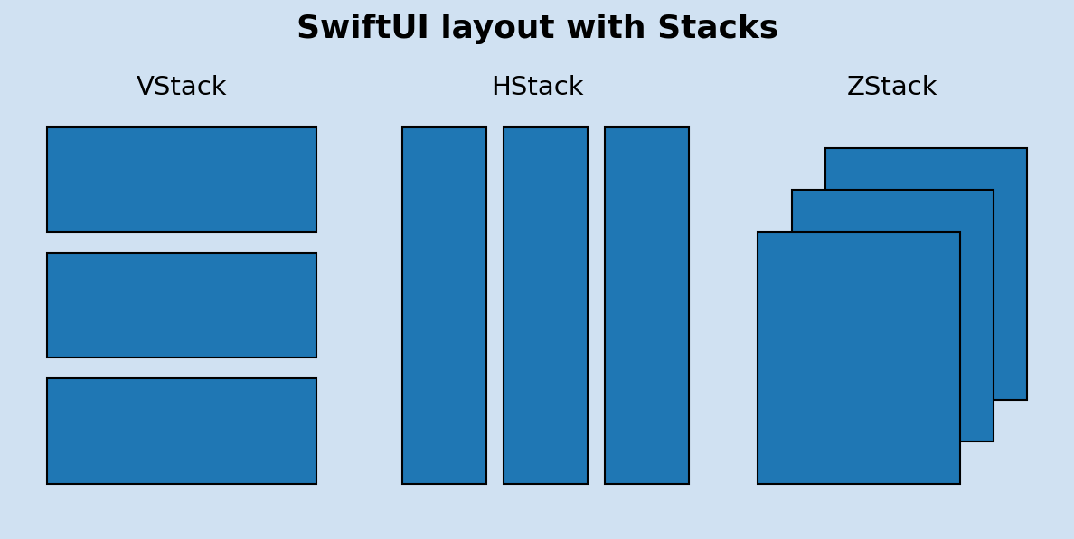
随着SwiftUI的出现,构建Apple平台应用的UI变得更为简洁和高效。本文从基础介绍开始,逐步深入到布局与组件的使用、数据绑定与状态管理、进阶功能的探究,最终达到项目实战的应用界面构建。本论文详细阐述了SwiftUI的核心概念、布局技巧、组件深度解析、动画与交互技术,以及响应式编程的实践。同时,探讨了SwiftUI在项目开发中的数据绑定原理、状态管理策略,并提供了进阶功
【IMS系统架构深度解析】:掌握关键组件与数据流

# 摘要
本文对IMS(IP多媒体子系统)系统架构及其核心组件进行了全面分析。首先概述了IMS系统架构,接着深入探讨了其核心组件如CSCF、MRF和SGW的角
【版本号自动生成工具探索】:第三方工具辅助Android项目版本自动化管理实用技巧

# 摘要
版本号自动生成工具是现代软件开发中不可或缺的辅助工具,它有助于提高项目管理效率和自动化程度。本文首先阐述了版本号管理的理论基础,强调了版本号的重要性及其在软件开发生命周期中的作用,并讨论了版本号的命名规则和升级策略。接着,详细介绍了版本号自动生成工具的选择、配置、使用以及实践案例分析,揭示了工具在自动化流程中的实际应用。进一步探讨了
【打印机小白变专家】:HL3160_3190CDW故障诊断全解析
# 摘要
本文系统地探讨了HL3160/3190CDW打印机的故障诊断与维护策略。首先介绍了打印机的基础知识,包括其硬件和软件组成及其维护重要性。接着,对常见故障进行了深入分析,覆盖了打印质量、操作故障以及硬件损坏等各类问题。文章详细阐述了故障诊断与解决方法,包括利用自检功能、软件层面的问题排查和硬件层面的维修指南。此外,本文还介绍了如何制定维护计划、性能监控和优化策略。通过案例研究和实战技巧的分享,提供了针对性的故障解决方案和维护优化的最佳实践。本文旨在为技术维修人员提供一份全面的打印机维护与故障处理指南,以提高打印机的可靠性和打印效率。
# 关键字
打印机故障;硬件组成;软件组件;维护计
逆变器滤波器设计:4个步骤降低噪声提升效率
# 摘要
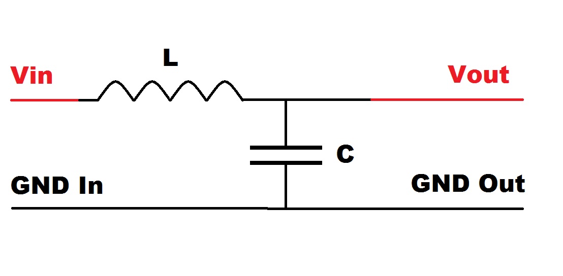
逆变器滤波器的设计是确保电力电子系统高效、可靠运作的关键因素之一。本文首先介绍了逆变器滤波器设计的基础知识,进而分析了噪声源对逆变器性能的影响以及滤波器在抑制噪声中的重要作用。文中详细阐述了逆变器滤波器设计的步骤,包括设计指标的确定、参数选择、模拟与仿真。通过具体的设计实践和案例分析,本文展示了滤波器的设计过程和搭建测试方法,并探讨了设计优化与故障排除的策略。最后,文章展望了滤波器设计领域未来的发展趋势
【Groovy社区与资源】:最新动态与实用资源分享指南

# 摘要
Groovy语言作为Java平台上的动态脚本语言,提供了灵活性和简洁性,能够大幅提升开发效率和程序的可读性。本文首先介绍Groovy的基本概念和核心特性,包括数据类型、控制结构、函数和闭包,以及如何利用这些特性简化编程模型。随后,文章探讨了Groovy脚本在自动化测试中的应用,特别是单元测试框架Spock的使用。进一步,文章详细分析了Groovy与S
【bat脚本执行不露声色】:专家揭秘CMD窗口隐身术

# 摘要
本论文深入探讨了CMD命令提示符及Bat脚本的基础知识、执行原理、窗口控制技巧、高级隐身技术,并通过实践应用案例展示了如何打造隐身脚本。文中详细介绍了批处理文件的创建、常用命令参数、执行环境配置、错误处理、CMD窗口外观定制以及隐蔽命令执行等
【VBScript数据类型与变量管理】:变量声明、作用域与生命周期探究,让你的VBScript更高效
# 摘要
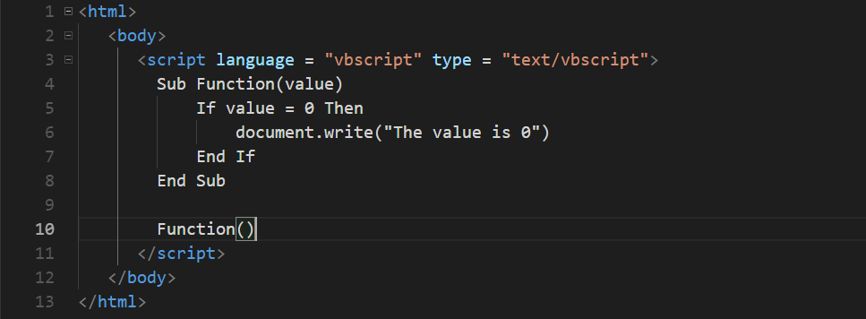
本文系统地介绍了VBScript数据类型、变量声明和初始化、变量作用域与生命周期、高级应用以及实践案例分析与优化技巧。首先概述了VBScript支持的基本和复杂数据类型,如字符串、整数、浮点数、数组、对象等,并详细讨论了变量的声明、初始化、赋值及类型转换。接着,分析了变量的作用域和生命周期,包括全局与局部变量的区别
资源上传下载、课程学习等过程中有任何疑问或建议,欢迎提出宝贵意见哦~我们会及时处理!
点击此处反馈


专栏目录
最低0.47元/天 解锁专栏
买1年送3月
百万级
高质量VIP文章无限畅学
千万级
优质资源任意下载
C知道
免费提问 ( 生成式Al产品 )