MATLAB Genetic Algorithm Visualization Tips: Visually Present the Optimization Process, Unveil the Secrets of Optimization
发布时间: 2024-09-15 04:49:02 阅读量: 29 订阅数: 36 
# 1. Introduction to MATLAB Genetic Algorithm
Genetic Algorithm (GA) is an optimization algorithm inspired by biological evolution, which simulates the processes of natural selection and genetic variation. GA iteratively searches for the optimal solution through the following steps:
- **Initialize Population:** Randomly generate a set of candidate solutions (called individuals).
- **Evaluate Fitness:** Calculate the fitness value of each individual, which reflects its adaptability to the optimization objective.
- **Selection:** Select the most suitable individuals for reproduction based on fitness values.
- **Crossover:** Cross the selected individuals to produce new offspring.
- **Mutation:** Randomly mutate the new offspring to introduce diversity.
- **Repeat:** Repeat steps 2-5 until the termination condition is met (e.g., reaching the maximum number of iterations or no further improvement in fitness values).
# 2.1 Visualizing Population Diversity
### 2.1.1 Population Distribution Plot
The population distribution plot shows the distribution of individuals in the population, reflecting the population's diversity. It helps us understand the convergence of the population and whether local optimum solutions exist.
**Code Block:**
```matlab
% Assuming a population size of 100, with each individual having 2 genes
population = rand(100, 2);
% Calculate the fitness of each individual
fitness = sum(population.^2, 2);
% Create the population distribution plot
figure;
scatter(population(:, 1), population(:, 2), [], fitness);
xlabel('Gene 1');
ylabel('Gene 2');
colorbar('title', 'Fitness');
```
**Logical Analysis:**
* `rand(100, 2)` generates a 100x2 random matrix representing 100 individuals in the population, each with 2 genes.
* `sum(population.^2, 2)` calculates the fitness of each individual, where `.^2` indicates element-wise squaring.
* The `scatter` function plots the population distribution, where `[]` indicates the use of the default colormap, and `fitness` indicates using fitness values as the colormap.
### 2.1.2 Population Convergence Curve
The population convergence curve shows how the population's fitness changes with the number of iterations during the optimization process. It helps us determine the convergence speed and stability of the optimization algorithm.
**Code Block:**
```matlab
% Assuming the optimization algorithm has run for 100 iterations
num_iterations = 100;
% Initialize the fitness array
fitness_array = zeros(1, num_iterations);
% Run the optimization algorithm and record the fitness
for i = 1:num_iterations
% ... optimization algorithm code ...
fitness_array(i) = ... fitness calculation ...
end
% Create the population convergence curve
figure;
plot(1:num_iterations, fitness_array);
xlabel('Number of Iterations');
ylabel('Fitness');
```
**Logical Analysis:**
* `zeros(1, num_iterations)` initializes a 1x`num_iterations` zero matrix to store fitness values.
* The optimization algorithm code is omitted, assuming the optimization algorithm has been implemented and the fitness is calculated in each iteration.
* The `plot` function plots the population convergence curve, where `1:num_iterations` represents the iteration number, and `fitness_array` represents the fitness values.
# 3. Visualization in Practice with Genetic Algorithm
### 3.1 Visualizing the Optimization Process of Traveling Salesman Problem
The Traveling Salesman Problem (TSP) is a classic combinatorial optimization problem where the goal is to find the shortest possible route that visits each city and returns to the starting point. Genetic algorithms can effectively solve TSP, and visualization techniques can help us understand the optimization process intuitively.
#### 3.1.1 Population Distribution Plot
The population distribution plot shows the distribution of individuals in the population. In TSP, each individual represents a path, and the individual's fitness is determined by the total distance of the path. By plotting the population distribution plot, we can observe the population's diversity and the convergence during the optimization process.
```matlab
% Generate an instance of the Traveling Salesman Problem
numCities = 10;
distances = rand(numCities);
distances = distances + distances';
distances(eye(numCities) == 1) = Inf;
% Genetic algorithm parameter settings
populationSize = 100;
maxGenerations = 100;
% Run the genetic algorithm
[bestPath, bestDistance] = ga(@(path) tspfun(path, distances), numCities, [], [], [], [], 1:numCities, [], [], gaoptimset('PopulationSize', populationSize, 'Generations', maxGenerations, 'PlotFcns', @gaplotbestf));
% Plot the population distribution
figure;
scatter(bestPath, bestDistance);
xlabel('Generation');
ylabel('Best Distance');
title('TSP Population Distribution');
```
#### 3.1.2 Optimization Trajectory Plot
The optimization trajectory plot shows the search trajectory of the genetic algorithm during the optimization process. In TSP, the optimization trajectory plot displays the change in the best path over time. By observing the optimization trajectory

 百万级
高质量VIP文章无限畅学
百万级
高质量VIP文章无限畅学
 千万级
优质资源任意下载
千万级
优质资源任意下载
 C知道
免费提问 ( 生成式Al产品 )
C知道
免费提问 ( 生成式Al产品 )
0
0
相关推荐

专栏目录
最低0.47元/天 解锁专栏
买1年送3月
百万级
高质量VIP文章无限畅学
千万级
优质资源任意下载
C知道
免费提问 ( 生成式Al产品 )
最新推荐
扇形菜单高级应用

# 摘要
扇形菜单作为一种创新的用户界面设计方式,近年来在多个应用领域中显示出其独特优势。本文概述了扇形菜单设计的基本概念和理论基础,深入探讨了其用户交互设计原则和布局算法,并介绍了其在移动端、Web应用和数据可视化中的应用案例
C++ Builder高级特性揭秘:探索模板、STL与泛型编程

# 摘要
本文系统性地介绍了C++ Builder的开发环境设置、模板编程、标准模板库(STL)以及泛型编程的实践与技巧。首先,文章提供了C++ Builder的简介和开发环境的配置指导。接着,深入探讨了C++模板编程的基础知识和高级特性,包括模板的特化、非类型模板参数以及模板
【深入PID调节器】:掌握自动控制原理,实现系统性能最大化

# 摘要
PID调节器是一种广泛应用于工业控制系统中的反馈控制器,它通过比例(P)、积分(I)和微分(D)三种控制作用的组合来调节系统的输出,以实现对被控对象的精确控制。本文详细阐述了PID调节器的概念、组成以及工作原理,并深入探讨了PID参数调整的多种方法和技巧。通过应用实例分析,本文展示了PID调节器在工业过程控制中的实际应用,并讨
【Delphi进阶高手】:动态更新百分比进度条的5个最佳实践

# 摘要
本文针对动态更新进度条在软件开发中的应用进行了深入研究。首先,概述了进度条的基础知识,然后详细分析了在Delphi环境下进度条组件的实现原理、动态更新机制以及多线程同步技术。进一步,文章探讨了数据处理、用户界面响应性优化和状态视觉呈现的实践技巧,并提出了进度
【TongWeb7架构深度剖析】:架构原理与组件功能全面详解
# 摘要
TongWeb7作为一个复杂的网络应用服务器,其架构设计、核心组件解析、性能优化、安全性机制以及扩展性讨论是本文的主要内容。本文首先对TongWeb7的架构进行了概述,然后详细分析了其核心中间件组件的功能与特点,接着探讨了如何优化性能监控与分析、负载均衡、缓存策略等方面,以及安全性机制中的认证授权、数据加密和安全策略实施。最后,本文展望
【S参数秘籍解锁】:掌握驻波比与S参数的终极关系
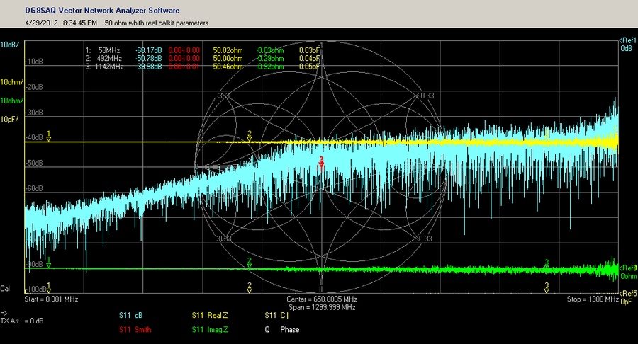
# 摘要
本论文详细阐述了驻波比与S参数的基础理论及其在微波网络中的应用,深入解析了S参数的物理意义、特性、计算方法以及在电路设计中的实践应用。通过分析S参数矩阵的构建原理、测量技术及仿真验证,探讨了S参数在放大器、滤波器设计及阻抗匹配中的重要性。同时,本文还介绍了驻波比的测量、优化策略及其与S参数的互动关系。最后,论文探讨了S参数分析工具的使用、高级分析技巧,并展望
【嵌入式系统功耗优化】:JESD209-5B的终极应用技巧
# 摘要
本文首先概述了嵌入式系统功耗优化的基本情况,随后深入解析了JESD209-5B标准,重点探讨了该标准的框架、核心规范、低功耗技术及实现细节。接着,本文奠定了功耗优化的理论基础,包括功耗的来源、分类、测量技术以及系统级功耗优化理论。进一步,本文通过实践案例深入分析了针对JESD209-5B标准的硬件和软件优化实践,以及不同应用场景下的功耗优化分析。最后,展望了未来嵌入式系统功耗优化的趋势,包括新兴技术的应用、JESD209-5B标准的发展以及绿色计算与可持续发展的结合,探讨了这些因素如何对未来的功耗优化技术产生影响。
# 关键字
嵌入式系统;功耗优化;JESD209-5B标准;低功耗
ODU flex接口的全面解析:如何在现代网络中最大化其潜力
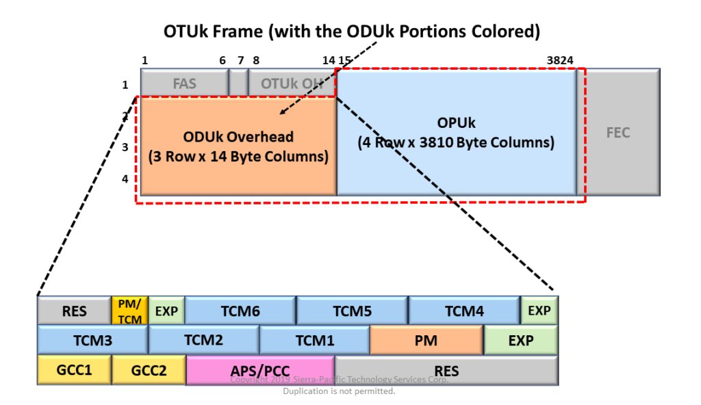
# 摘要
ODU flex接口作为一种高度灵活且可扩展的光传输技术,已经成为现代网络架构优化和电信网络升级的重要组成部分。本文首先概述了ODU flex接口的基本概念和物理层特征,紧接着深入分析了其协议栈和同步机制,揭示了其在数据中心、电信网络、广域网及光纤网络中的应用优势和性能特点。文章进一步
如何最大化先锋SC-LX59的潜力
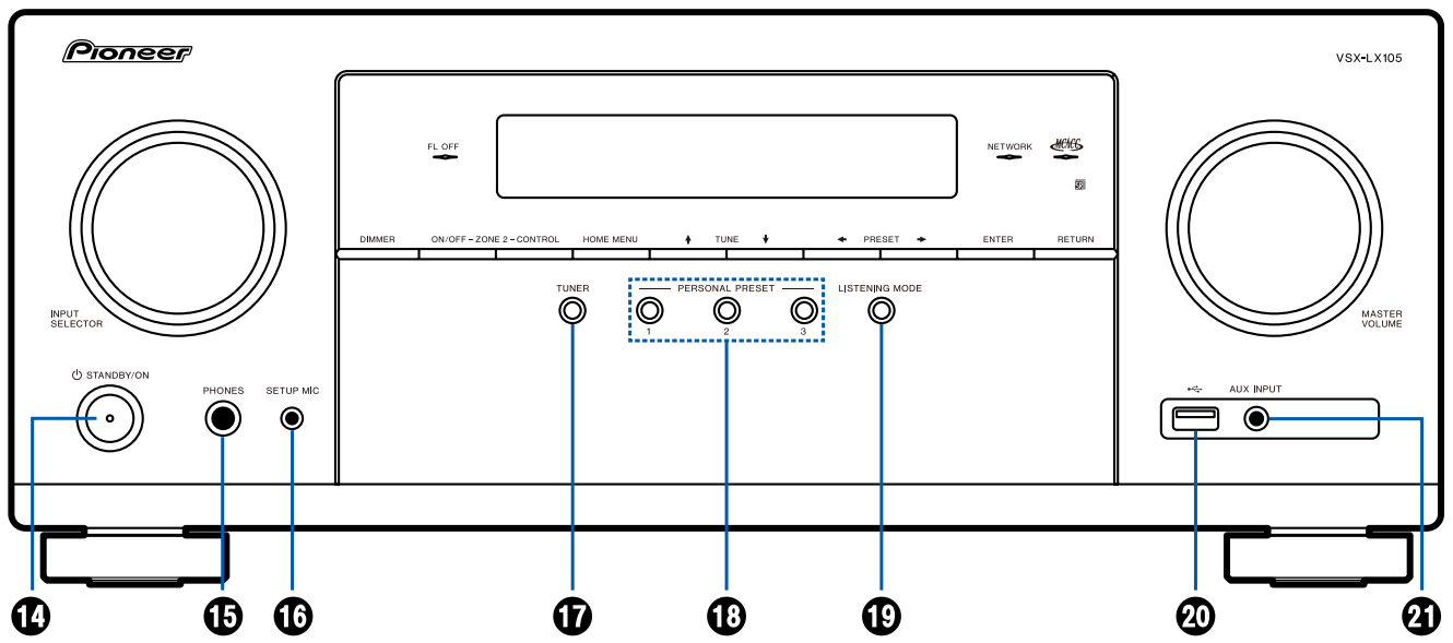
# 摘要
先锋SC-LX59作为一款高端家庭影院接收器,其在音视频性能、用户体验、网络功能和扩展性方面均展现出巨大的潜力。本文首先概述了SC-LX59的基本特点和市场潜力,随后深入探讨了其设置与配置的最佳实践,包括用户界面的个性化和音画效果的调整,连接选项与设备兼容性,以及系统性能的调校。第三章着重于先锋SC-LX59在家庭影院中的应用,特别强调了音视频极致体验、智能家居集成和流媒体服务的充分利用。在高
资源上传下载、课程学习等过程中有任何疑问或建议,欢迎提出宝贵意见哦~我们会及时处理!
点击此处反馈


专栏目录
最低0.47元/天 解锁专栏
买1年送3月
百万级
高质量VIP文章无限畅学
千万级
优质资源任意下载
C知道
免费提问 ( 生成式Al产品 )