MATLAB Genetic Algorithm and Machine Learning Integration Guide: Enhancing Optimization Algorithms, Improving Performance
发布时间: 2024-09-15 05:00:36 阅读量: 14 订阅数: 13 
# MATLAB Genetic Algorithm and Machine Learning Integration Guide: Enhancing Optimization Algorithms and Improving Performance
## 1. Overview of Machine Learning and Genetic Algorithms
### 1.1 Introduction to Machine Learning
Machine learning is an artificial intelligence technique that enables computers to learn from data without explicit programming. Machine learning algorithms can recognize patterns, predict outcomes, and make decisions.
### 1.2 Introduction to Genetic Algorithms
Genetic algorithms are optimization algorithms inspired by the theory of evolution. They simulate the process of natural selection, optimizing solutions through operations of crossover, mutation, and selection.
## 2.1 Basics of Genetic Algorithms
### 2.1.1 Principles of Genetic Algorithms
Genetic algorithms are heuristic search algorithms that simulate the process of biological evolution in nature to solve optimization problems. Their basic principles are:
***Population Initialization:** Randomly generate a population consisting of multiple individuals, each representing a potential solution.
***Fitness Calculation:** Calculate the fitness value of each individual based on its fitness function (a measure of individual quality).
***Selection:** Select superior individuals for the next generation based on their fitness values.
***Crossover:** Combine two or more parent individuals to generate new offspring individuals.
***Mutation:** Introduce variety by randomly mutating offspring individuals.
***Iteration:** Repeat the above steps until a predetermined termination condition is met (e.g., maximum iterations or achieving an optimal solution).
### 2.1.2 Flow of Genetic Algorithms
The flow of genetic algorithms can be summarized as follows:
1. **Problem Modeling:** Convert the optimization problem into a genetic algorithm problem, defining the fitness function and population encoding.
2. **Population Initialization:** Generate the initial population.
3. **Fitness Calculation:** Calculate the fitness value of each individual.
4. **Selection:** Select superior individuals for the next generation population.
5. **Crossover:** Perform crossover on parent individuals.
6. **Mutation:** Mutate offspring individuals.
7. **Repeat Steps 3-6:** Repeat the above steps until the termination condition is met.
8. **Output:** Output the best individual or population.
**Code Block:**
```matlab
% Genetic Algorithm Process
function [best_individual, best_fitness] = genetic_algorithm(problem, options)
% Initialize population
population = initialize_population(problem, options.population_size);
% Iterative evolution
for i = 1:options.max_iterations
% Calculate fitness
fitness = evaluate_fitness(population, problem);
% Selection
selected_individuals = select_individuals(population, fitness, options.selection_method);
% Crossover
new_population = crossover(selected_individuals, options.crossover_method);
% Mutation
new_population = mutate(new_population, options.mutation_rate);
% Update population
population = new_population;
end
% Output the best individual
[best_fitness, best_individual_index] = max(fitness);
best_individual = population(best_individual_index);
end
```
**Logical Analysis:**
This code implements the basic flow of genetic algorithms. It initializes the population, iteratively evolves, and calculates fitness, selects individuals, and performs crossover and mutation in each iteration. Finally, it outputs the best individual and optimal fitness value.
**Parameter Explanation:**
* `problem`: The optimization problem, including the fitness function and population encoding.
* `options`: Genetic algorithm options, including population size, maximum iterations, selection method, crossover method, and mutation rate.
## 3. Implementation of Genetic Algorithms in MATLAB
### 3.1 MATLAB Genetic Algorithm Toolbox
MATLAB provides a series of genetic algorithm toolboxes, ***o commonly used functions are:
- **ga function:** Used for solving single-objective optimization problems.
- **gamultiobj function:** Used for solving multi-objective optimization problems.
#### 3.1.1 ga Function
**Parameter Explanation:**
| Parameter | Description |
|---|---|
| `fitnessfcn` | Objective function handle |
| `nvars` | Number of decision variables |
| `Aineq` | Linear inequality constraint matrix |
| `bineq` | Linear inequality constraint vector |
| `Aeq` | Linear equality constraint matrix |
| `beq` | Linear equality constraint vector |
| `lb` | Lower bound of decision variables |
| `ub` | Upper bound of decision variables |
**Code Block:**
```
% Objective Function
fitnessfcn = @(x) -x(1)^2 - x(2)^2;
% Number of Decision Variables
nvars = 2;
% Genetic Algorithm Options
options = gaoptimset('PopulationSize', 100, 'Generations', 100);
% Run Genetic Algorithm
[x, fval] = ga(fitnessfcn, nvars, [], [], [], [], [], [], [], options);
```
**Logical Analysis:**
This code block uses the ga function to solve a single-objective optimization problem. The objective function is a quadratic function, and the number of decision variables is 2. Genetic algorithm options set the population size to 100 and the number of generations to 100.
#### 3.1.2 gamultiobj Function
**Parameter Explanation:**
| Parameter | Description |
|---|---|
| `fitnessfcn` | Objective function handle |
| `nvars` | Number of decision variables |
| `Aineq` | Linear inequality constraint matrix |
| `bineq` | Linear inequality constraint vector |
| `Aeq` | Linear equality constraint matrix |
| `beq` | Linear equality constraint vector |
| `lb` | Lower bound of decision variables |
| `ub` | Upper bound of decision variables |
| `options` | Genetic algorithm options
 最低0.47元/天 解锁专栏
 送3个月
 百万级
高质量VIP文章无限畅学
百万级
高质量VIP文章无限畅学
 千万级
优质资源任意下载
千万级
优质资源任意下载
 C知道
免费提问 ( 生成式Al产品 )
C知道
免费提问 ( 生成式Al产品 )
0
0
相关推荐

专栏目录
最低0.47元/天 解锁专栏
送3个月
百万级
高质量VIP文章无限畅学
千万级
优质资源任意下载
C知道
免费提问 ( 生成式Al产品 )
最新推荐
Python版本与性能优化:选择合适版本的5个关键因素

# 1. Python版本选择的重要性
Python是不断发展的编程语言,每个新版本都会带来改进和新特性。选择合适的Python版本至关重要,因为不同的项目对语言特性的需求差异较大,错误的版本选择可能会导致不必要的兼容性问题、性能瓶颈甚至项目失败。本章将深入探讨Python版本选择的重要性,为读者提供选择和评估Python版本的决策依据。
Python的版本更新速度和特性变化需要开发者们保持敏锐的洞
【Python集合异常处理攻略】:集合在错误控制中的有效策略
# 1. Python集合的基础知识
Python集合是一种无序的、不重复的数据结构,提供了丰富的操作用于处理数据集合。集合(set)与列表(list)、元组(tuple)、字典(dict)一样,是Python中的内置数据类型之一。它擅长于去除重复元素并进行成员关系测试,是进行集合操作和数学集合运算的理想选择。
集合的基础操作包括创建集合、添加元素、删除元素、成员测试和集合之间的运
Python序列化与反序列化高级技巧:精通pickle模块用法

# 1. Python序列化与反序列化概述
在信息处理和数据交换日益频繁的今天,数据持久化成为了软件开发中不可或缺的一环。序列化(Serialization)和反序列化(Deserialization)是数据持久化的重要组成部分,它们能够将复杂的数据结构或对象状态转换为可存储或可传输的格式,以及还原成原始数据结构的过程。
序列化通常用于数据存储、
【Python数组的内存管理】:引用计数和垃圾回收的高级理解
# 1. Python数组的内存分配基础
在探讨Python的数组内存分配之前,首先需要对Python的对象模型有一个基本的认识。Python使用一种称为“动态类型系统”的机制,它允许在运行时动态地分配和管理内存。数组作为一种序列类型,在Python中通常使用列表(list)来实现,而列表则是通过动态数组或者叫做数组列表(array list)的数据结构来实现内存管理的。每个P
Python print语句装饰器魔法:代码复用与增强的终极指南

# 1. Python print语句基础
## 1.1 print函数的基本用法
Python中的`print`函数是最基本的输出工具,几乎所有程序员都曾频繁地使用它来查看变量值或调试程序。以下是一个简单的例子来说明`print`的基本用法:
```python
print("Hello, World!")
```
这个简单的语句会输出字符串到标准输出,即你的控制台或终端。`prin
Pandas中的文本数据处理:字符串操作与正则表达式的高级应用
# 1. Pandas文本数据处理概览
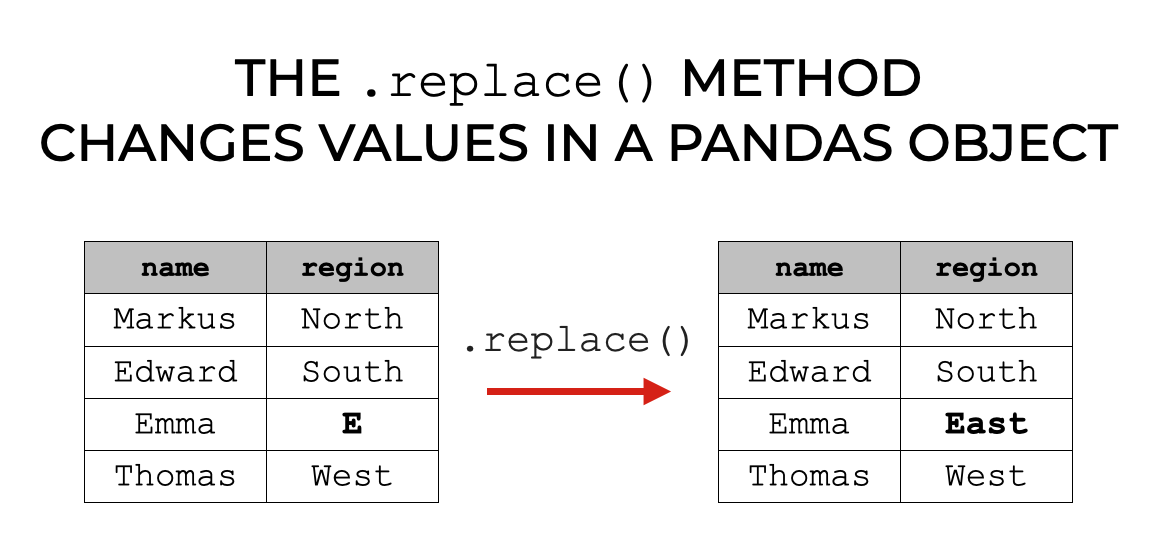
Pandas库不仅在数据清洗、数据处理领域享有盛誉,而且在文本数据处理方面也有着独特的优势。在本章中,我们将介绍Pandas处理文本数据的核心概念和基础应用。通过Pandas,我们可以轻松地对数据集中的文本进行各种形式的操作,比如提取信息、转换格式、数据清洗等。
我们会从基础的字
Python pip性能提升之道
# 1. Python pip工具概述
Python开发者几乎每天都会与pip打交道,它是Python包的安装和管理工具,使得安装第三方库变得像“pip install 包名”一样简单。本章将带你进入pip的世界,从其功能特性到安装方法,再到对常见问题的解答,我们一步步深入了解这一Python生态系统中不可或缺的工具。
首先,pip是一个全称“Pip Installs Pac
Image Processing and Computer Vision Techniques in Jupyter Notebook
# Image Processing and Computer Vision Techniques in Jupyter Notebook
## Chapter 1: Introduction to Jupyter Notebook
### 2.1 What is Jupyter Notebook
Jupyter Notebook is an interactive computing environment that supports code execution, text writing, and image display. Its main features include:
-
Parallelization Techniques for Matlab Autocorrelation Function: Enhancing Efficiency in Big Data Analysis
# 1. Introduction to Matlab Autocorrelation Function
The autocorrelation function is a vital analytical tool in time-domain signal processing, capable of measuring the similarity of a signal with itself at varying time lags. In Matlab, the autocorrelation function can be calculated using the `xcorr
Technical Guide to Building Enterprise-level Document Management System using kkfileview
# 1.1 kkfileview Technical Overview
kkfileview is a technology designed for file previewing and management, offering rapid and convenient document browsing capabilities. Its standout feature is the support for online previews of various file formats, such as Word, Excel, PDF, and more—allowing user
资源上传下载、课程学习等过程中有任何疑问或建议,欢迎提出宝贵意见哦~我们会及时处理!
点击此处反馈


专栏目录
最低0.47元/天 解锁专栏
送3个月
百万级
高质量VIP文章无限畅学
千万级
优质资源任意下载
C知道
免费提问 ( 生成式Al产品 )