[Practical Exercise] Gaussian Belief Propagation Algorithm for DC State Estimation Model in MATLAB
发布时间: 2024-09-14 00:27:41 阅读量: 10 订阅数: 37 
# 2.1 Principles of Gaussian Belief Propagation Algorithm
Gaussian Belief Propagation (GBP) is a nonlinear state estimation algorithm based on the Bayesian filtering framework. It approximates the posterior probability density function with non-Gaussian distributions using Gaussian distributions, thus achieving state estimation in nonlinear systems.
### 2.1.1 State Prediction and Update Equations
The core concept of the GBP algorithm is to update the state distribution through message passing. In the state prediction step, the prior distribution of the system state is updated to the posterior distribution through the transition probability density function:
```
p(x_k | y_{1:k-1}) = \int p(x_k | x_{k-1}) p(x_{k-1} | y_{1:k-1}) dx_{k-1}
```
Here, x_k represents the state at time k, y_{1:k-1} represents the observed data from time 1 to k-1, p(x_k | x_{k-1}) is the transition probability density function, and p(x_{k-1} | y_{1:k-1}) is the state posterior distribution at time k-1.
In the state update step, the posterior distribution is updated to a new posterior distribution through the observation probability density function:
```
p(x_k | y_{1:k}) = \frac{p(y_k | x_k) p(x_k | y_{1:k-1})}{\int p(y_k | x_k) p(x_k | y_{1:k-1}) dx_k}
```
Here, p(y_k | x_k) is the observation probability density function.
### 2.1.2 Weight Update Equations
In the GBP algorithm, the weight of each state variable represents its importance in the posterior distribution. The weight update equations are used to update the weights to reflect the credibility of the state variables under the observed data:
```
w_k(x_k) = \frac{p(y_k | x_k) w_{k-1}(x_k)}{\sum_{x_k} p(y_k | x_k) w_{k-1}(x_k)}
```
Here, w_k(x_k) represents the weight of state x_k at time k, and w_{k-1}(x_k) represents the weight at time k-1.
# 2. Gaussian Belief Propagation Theory
### 2.1 Principles of Gaussian Belief Propagation
Gaussian Belief Propagation (GBP) is an approximate reasoning algorithm used for nonlinear, non-Gaussian state estimation. Its basic principle is to use Gaussian distributions to approximate non-Gaussian distributions and propagate these Gaussian distributions to approximate the calculation of the posterior distribution.
#### 2.1.1 State Prediction and Update Equations
In the GBP algorithm, the system state is represented by a Gaussian distribution, namely:
```
p(x) = N(x; μ, Σ)
```
Here, μ and Σ represent the mean and covariance matrix of the Gaussian distribution, respectively.
In the state prediction phase, the state prediction distribution can be obtained based on the system model and prior distribution:
```
p(x_t | x_{t-1}) = N(x_t; f(x_{t-1}), Q)
```
Here, f(x_{t-1}) represents the system model, and Q represents the process noise covariance matrix.
In the state update phase, the state posterior distribution can be obtained based on the measurement model and prediction distribution:
```
p(x_t | y_t, x_{t-1}) = N(x_t; μ_t, Σ_t)
```
Here, μ_t and Σ_t represent the mean and covariance matrix of the posterior distribution, respectively, and the calculation formulas are:
```
μ_t = μ_t^- + K_t(y_t - h(μ_t^-))
Σ_t = Σ_t^- - K_tH_tΣ_t^-
```
Here, μ_t^- and Σ_t^- represent the mean and covariance matrix of the prediction distribution, respectively, K_t is the Kalman gain, and H_t is the Jacobian matrix of the measurement model.
#### 2.1.2 Weight Update Equations
In the GBP algorithm, each Gaussian distribution is associated with a weight representing its importance in the posterior distribution. The weight update equations are used to update these weights, and the formula is:
```
w_t = w_{t-1}N(y_t; h(μ_t), H_tΣ_tH_t^T + R)
```
Here, w_t and w_{t-1} represent the updated and previous weights, respectively, and R represents the measurement noise covariance matrix.
### 2.2 Advantages and Limitations of Gaussian Belief Propagation
#### 2.2.1 Advantages: Nonlinear, Non-Gaussian State Estimation
The advantage of the GBP algorithm is that it can be used for nonlinear, non-Gaussian state estimation. Traditional Kalman filters can only be used for linear, Gaussian systems, while the GBP algorithm approximates non-Gaussian distributions as Gaussian distributions, allowing it to handle more complex systems.
#### 2.2.2 Limitations: High Computational Load, Sensitive to Initial Conditions
The limitation of the GBP algorithm is that its computational load is high, especially when the system dimension is high. I
 最低0.47元/天 解锁专栏
 送3个月
 百万级
高质量VIP文章无限畅学
百万级
高质量VIP文章无限畅学
 千万级
优质资源任意下载
千万级
优质资源任意下载
 C知道
免费提问 ( 生成式Al产品 )
C知道
免费提问 ( 生成式Al产品 )
0
0
相关推荐

专栏目录
最低0.47元/天 解锁专栏
送3个月
百万级
高质量VIP文章无限畅学
千万级
优质资源任意下载
C知道
免费提问 ( 生成式Al产品 )
最新推荐
Python函数调用栈分析:追踪执行流程,优化函数性能的6个技巧

# 1. 函数调用栈基础
函数调用栈是程序执行过程中用来管理函数调用关系的一种数据结构,它类似于一叠盘子的堆栈,记录了程序从开始运行到当前时刻所有函数调用的序列。理解调用栈对于任何希望深入研究编程语言内部运行机制的开发者来说都是至关重要的,它能帮助你解决函数调用顺序混乱、内存泄漏以及性能优化等问题。
## 1.1 什么是调用栈
调用栈是一个后进先出(LIFO)的栈结构,用于记录函数调用的顺序和执行环境。
【Python集合异常处理攻略】:集合在错误控制中的有效策略
# 1. Python集合的基础知识
Python集合是一种无序的、不重复的数据结构,提供了丰富的操作用于处理数据集合。集合(set)与列表(list)、元组(tuple)、字典(dict)一样,是Python中的内置数据类型之一。它擅长于去除重复元素并进行成员关系测试,是进行集合操作和数学集合运算的理想选择。
集合的基础操作包括创建集合、添加元素、删除元素、成员测试和集合之间的运
【递归与迭代决策指南】:如何在Python中选择正确的循环类型
# 1. 递归与迭代概念解析
## 1.1 基本定义与区别
递归和迭代是算法设计中常见的两种方法,用于解决可以分解为更小、更相似问题的计算任务。**递归**是一种自引用的方法,通过函数调用自身来解决问题,它将问题简化为规模更小的子问题。而**迭代**则是通过重复应用一系列操作来达到解决问题的目的,通常使用循环结构实现。
## 1.2 应用场景
递归算法在需要进行多级逻辑处理时特别有用,例如树的遍历和分治算法。迭代则在数据集合的处理中更为常见,如排序算法和简单的计数任务。理解这两种方法的区别对于选择最合适的算法至关重要,尤其是在关注性能和资源消耗时。
## 1.3 逻辑结构对比
递归
Python数组在科学计算中的高级技巧:专家分享

# 1. Python数组基础及其在科学计算中的角色
数据是科学研究和工程应用中的核心要素,而数组作为处理大量数据的主要工具,在Python科学计算中占据着举足轻重的地位。在本章中,我们将从Python基础出发,逐步介绍数组的概念、类型,以及在科学计算中扮演的重要角色。
## 1.1 Python数组的基本概念
数组是同类型元素的有序集合,相较于Python的列表,数组在内存中连续存储,允
Python装饰模式实现:类设计中的可插拔功能扩展指南
# 1. Python装饰模式概述
装饰模式(Decorator Pattern)是一种结构型设计模式,它允许动态地添加或修改对象的行为。在Python中,由于其灵活性和动态语言特性,装饰模式得到了广泛的应用。装饰模式通过使用“装饰者”(Decorator)来包裹真实的对象,以此来为原始对象添加新的功能或改变其行为,而不需要修改原始对象的代码。本章将简要介绍Python中装饰模式的概念及其重要性,为理解后
【Python字典的并发控制】:确保数据一致性的锁机制,专家级别的并发解决方案

# 1. Python字典并发控制基础
在本章节中,我们将探索Python字典并发控制的基础知识,这是在多线程环境中处理共享数据时必须掌握的重要概念。我们将从了解为什么需要并发控制开始,然后逐步深入到Python字典操作的线程安全问题,最后介绍一些基本的并发控制机制。
## 1.1 并发控制的重要性
在多线程程序设计中
Python版本与性能优化:选择合适版本的5个关键因素

# 1. Python版本选择的重要性
Python是不断发展的编程语言,每个新版本都会带来改进和新特性。选择合适的Python版本至关重要,因为不同的项目对语言特性的需求差异较大,错误的版本选择可能会导致不必要的兼容性问题、性能瓶颈甚至项目失败。本章将深入探讨Python版本选择的重要性,为读者提供选择和评估Python版本的决策依据。
Python的版本更新速度和特性变化需要开发者们保持敏锐的洞
Python print语句装饰器魔法:代码复用与增强的终极指南

# 1. Python print语句基础
## 1.1 print函数的基本用法
Python中的`print`函数是最基本的输出工具,几乎所有程序员都曾频繁地使用它来查看变量值或调试程序。以下是一个简单的例子来说明`print`的基本用法:
```python
print("Hello, World!")
```
这个简单的语句会输出字符串到标准输出,即你的控制台或终端。`prin
Pandas中的文本数据处理:字符串操作与正则表达式的高级应用
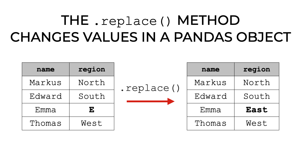
# 1. Pandas文本数据处理概览
Pandas库不仅在数据清洗、数据处理领域享有盛誉,而且在文本数据处理方面也有着独特的优势。在本章中,我们将介绍Pandas处理文本数据的核心概念和基础应用。通过Pandas,我们可以轻松地对数据集中的文本进行各种形式的操作,比如提取信息、转换格式、数据清洗等。
我们会从基础的字
Python pip性能提升之道
# 1. Python pip工具概述
Python开发者几乎每天都会与pip打交道,它是Python包的安装和管理工具,使得安装第三方库变得像“pip install 包名”一样简单。本章将带你进入pip的世界,从其功能特性到安装方法,再到对常见问题的解答,我们一步步深入了解这一Python生态系统中不可或缺的工具。
首先,pip是一个全称“Pip Installs Pac
资源上传下载、课程学习等过程中有任何疑问或建议,欢迎提出宝贵意见哦~我们会及时处理!
点击此处反馈


专栏目录
最低0.47元/天 解锁专栏
送3个月
百万级
高质量VIP文章无限畅学
千万级
优质资源任意下载
C知道
免费提问 ( 生成式Al产品 )